Adaptive Evolution climbing the fitness landscape Outline where

Adaptive Evolution: climbing the fitness landscape

Outline: where are we and where are we going? Last few lectures focused exclusively on deleterious mutations (s < 0) • single locus, deterministic: frequency of deleterious allele = u/s. • multi-locus: SEVERAL deleterious alleles present in population. • fraction of population carrying k mutations is Poisson w/ mean U/s • mean # mutations in population = U/s • mean fitness in population = e-U ≈ 1 -U (“deleterious load” = U) Next three lectures we will focus exclusively on beneficial mutations (s > 0): how fast can populations adapt? (“the theory of change”) • regime when beneficial mutations are rare (math ≈ “easy”) • regime when beneficial mutations are common (math = much harder) What are realistic values for “population size” (N)? What does N really mean? • definition of Ne: “effective population size” • introduction to coalescent theory • how Ne is measured • factors influencing Ne

The basic problem: how fast can populations increase their fitness? In the simplest case, there are just 3 parameters: • Ub = “beneficial mutation rate”, per genome per generation • s = selection coefficient (advantage) of new beneficial mutations • N = population size (census) Note: we’re leaving out tons of things • deleterious mutations • variation in s (some beneficial muts. are stronger than others) • possibility of environmental change These omissions are all interesting, but you have to walk before you can run… The thing we want to calculate is the speed of evolution, v(Ub, s, N). Clicker question: According to your intuitions, does v increase or decrease with: increase • Ub increase • s • N increase

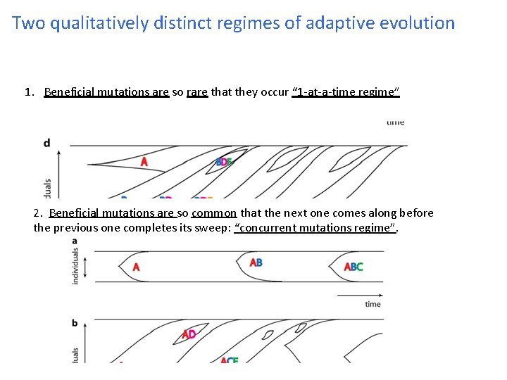
Two qualitatively distinct regimes of adaptive evolution 1. Beneficial mutations are so rare that they occur “ 1 -at-a-time regime” 2. Beneficial mutations are so common that the next one comes along before the previous one completes its sweep: “concurrent mutations regime”.

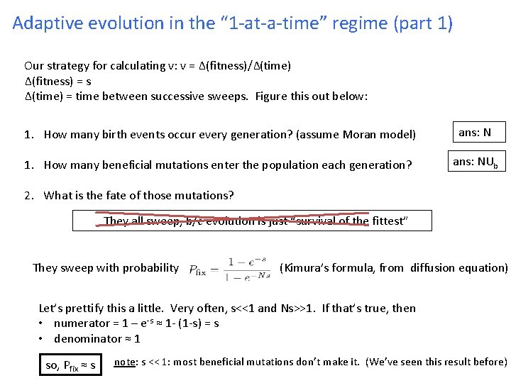
Adaptive evolution in the “ 1 -at-a-time” regime (part 1) Our strategy for calculating v: v = Δ(fitness)/Δ(time) Δ(fitness) = s Δ(time) = time between successive sweeps. Figure this out below: 1. How many birth events occur every generation? (assume Moran model) ans: N 1. How many beneficial mutations enter the population each generation? ans: NUb 2. What is the fate of those mutations? They all sweep, b/c evolution is just “survival of the fittest” They sweep with probability (Kimura’s formula, from diffusion equation) Let’s prettify this a little. Very often, s<<1 and Ns>>1. If that’s true, then • numerator = 1 – e-s ≈ 1 - (1 -s) = s • denominator ≈ 1 so, Pfix ≈ s note: s << 1: most beneficial mutations don’t make it. (We’ve seen this result before)

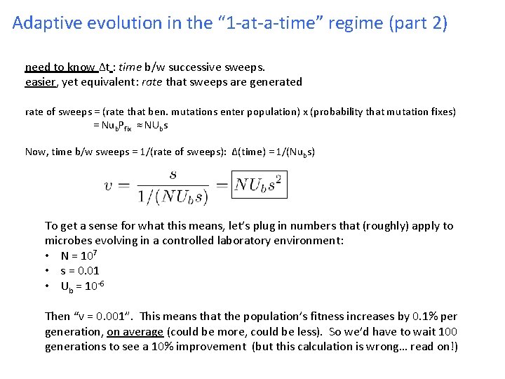
Adaptive evolution in the “ 1 -at-a-time” regime (part 2) need to know Δt : time b/w successive sweeps. easier, yet equivalent: rate that sweeps are generated rate of sweeps = (rate that ben. mutations enter population) x (probability that mutation fixes) = Nub. Pfix ≈ NUbs Now, time b/w sweeps = 1/(rate of sweeps): Δ(time) = 1/(Nubs) To get a sense for what this means, let’s plug in numbers that (roughly) apply to microbes evolving in a controlled laboratory environment: • N = 107 • s = 0. 01 • Ub = 10 -6 Then “v = 0. 001”. This means that the population’s fitness increases by 0. 1% per generation, on average (could be more, could be less). So we’d have to wait 100 generations to see a 10% improvement (but this calculation is wrong… read on!)

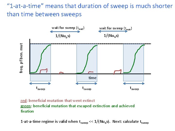
“ 1 -at-a-time” means that duration of sweep is much shorter than time between sweeps wait for sweep (twait) 1/(Nubs) freq. pf ben. mut 1/(Nubs) time tsweep red: beneficial mutation that went extinct green: beneficial mutation that escaped extinction and achieved fixation 1 -at-a-time regime is valid when tsweep << 1/(Nubs). Next: calculate ttweep

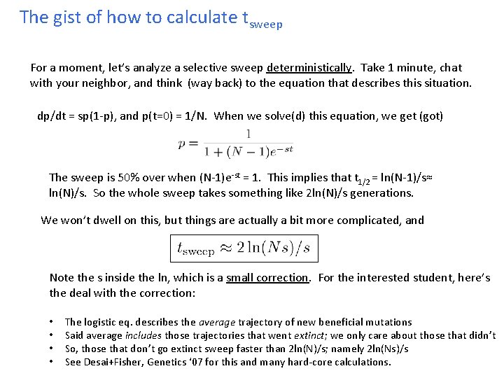
The gist of how to calculate tsweep For a moment, let’s analyze a selective sweep deterministically. Take 1 minute, chat with your neighbor, and think (way back) to the equation that describes this situation. dp/dt = sp(1 -p), and p(t=0) = 1/N. When we solve(d) this equation, we get (got) The sweep is 50% over when (N-1)e-st = 1. This implies that t 1/2 = ln(N-1)/s≈ ln(N)/s. So the whole sweep takes something like 2 ln(N)/s generations. We won’t dwell on this, but things are actually a bit more complicated, and Note the s inside the ln, which is a small correction. For the interested student, here’s the deal with the correction: • • The logistic eq. describes the average trajectory of new beneficial mutations Said average includes those trajectories that went extinct; we only care about those that didn’t So, those that don’t go extinct sweep faster than 2 ln(N)/s; namely 2 ln(Ns)/s See Desai+Fisher, Genetics ‘ 07 for this and many hard-core calculations.

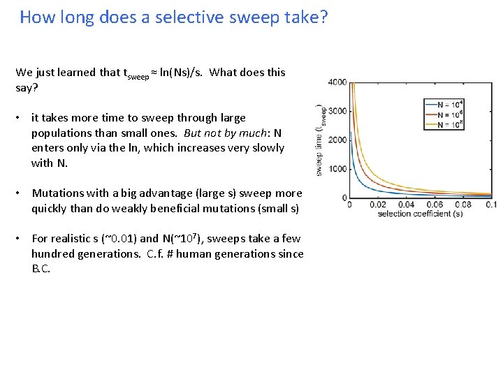
How long does a selective sweep take? We just learned that tsweep ≈ ln(Ns)/s. What does this say? • it takes more time to sweep through large populations than small ones. But not by much: N enters only via the ln, which increases very slowly with N. • Mutations with a big advantage (large s) sweep more quickly than do weakly beneficial mutations (small s) • For realistic s (~0. 01) and N(~107), sweeps take a few hundred generations. C. f. # human generations since B. C.

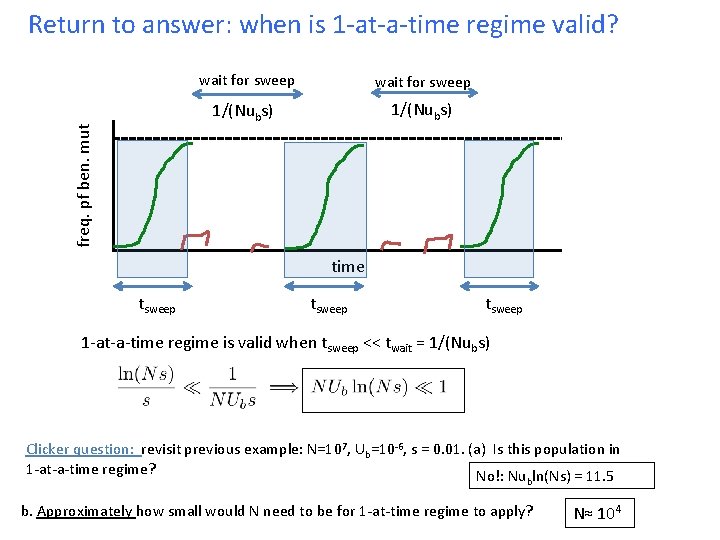
freq. pf ben. mut Return to answer: when is 1 -at-a-time regime valid? wait for sweep 1/(Nubs) time tsweep 1 -at-a-time regime is valid when tsweep << twait = 1/(Nubs) Clicker question: revisit previous example: N=107, Ub=10 -6, s = 0. 01. (a) Is this population in 1 -at-a-time regime? No!: Nu ln(Ns) = 11. 5 b b. Approximately how small would N need to be for 1 -at-time regime to apply? N≈ 104

Closing thoughts and preview for next time… • We just saw that the 1 -at-a-time regime does not apply to for “typical” laboratory populations of microbes. It probably does not apply to “wild” populations either. • The population size (N) plays a huge role in determining whether or not the 1 -at-a time regime applies. So giant question: what is N in the wild? What does N really mean (we’ll consider this on Friday) • Tomorrow we’ll consider how fast populations adapt in the “concurrent mutations regime”.