Adaptive Algorithms for PCA Review of Principal Component

Adaptive Algorithms for PCA

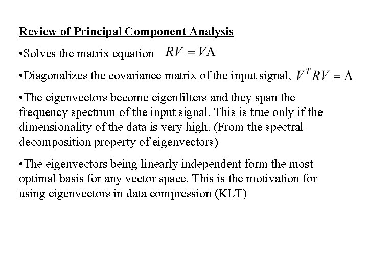
Review of Principal Component Analysis • Solves the matrix equation • Diagonalizes the covariance matrix of the input signal, • The eigenvectors become eigenfilters and they span the frequency spectrum of the input signal. This is true only if the dimensionality of the data is very high. (From the spectral decomposition property of eigenvectors) • The eigenvectors being linearly independent form the most optimal basis for any vector space. This is the motivation for using eigenvectors in data compression (KLT)

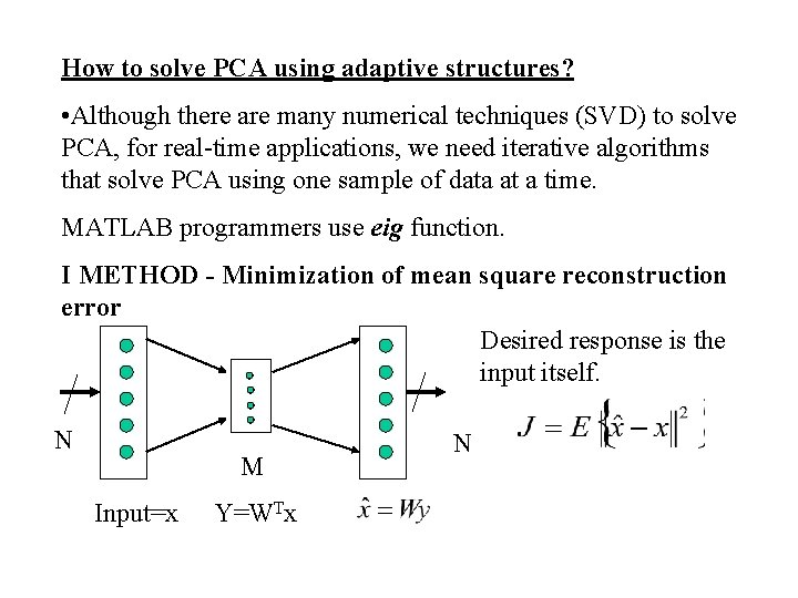
How to solve PCA using adaptive structures? • Although there are many numerical techniques (SVD) to solve PCA, for real-time applications, we need iterative algorithms that solve PCA using one sample of data at a time. MATLAB programmers use eig function. I METHOD - Minimization of mean square reconstruction error Desired response is the input itself. N M Input=x Y=WTx N

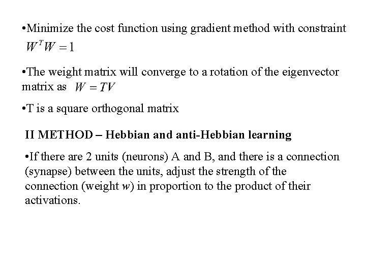
• Minimize the cost function using gradient method with constraint • The weight matrix will converge to a rotation of the eigenvector matrix as • T is a square orthogonal matrix II METHOD – Hebbian and anti-Hebbian learning • If there are 2 units (neurons) A and B, and there is a connection (synapse) between the units, adjust the strength of the connection (weight w) in proportion to the product of their activations.

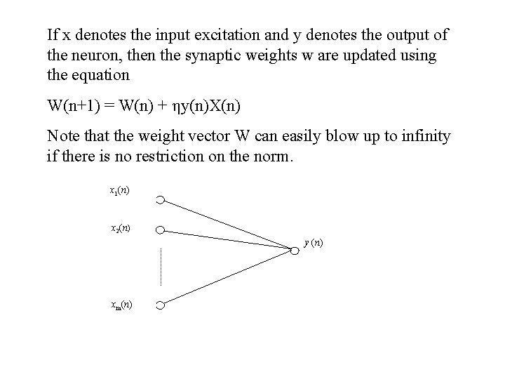
If x denotes the input excitation and y denotes the output of the neuron, then the synaptic weights w are updated using the equation W(n+1) = W(n) + ηy(n)X(n) Note that the weight vector W can easily blow up to infinity if there is no restriction on the norm. x 1(n) x 2(n) y (n) xm(n)

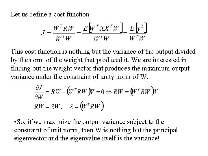
Let us define a cost function This cost function is nothing but the variance of the output divided by the norm of the weight that produced it. We are interested in finding out the weight vector that produces the maximum output variance under the constraint of unity norm of W. • So, if we maximize the output variance subject to the constraint of unit norm, then W is nothing but the principal eigenvector and the eigenvalue itself is the variance!

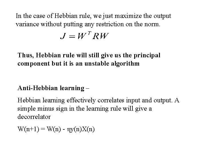
In the case of Hebbian rule, we just maximize the output variance without putting any restriction on the norm. Thus, Hebbian rule will still give us the principal component but it is an unstable algorithm Anti-Hebbian learning – Hebbian learning effectively correlates input and output. A simple minus sign in the learning rule will give a decorrelator W(n+1) = W(n) - ηy(n)X(n)

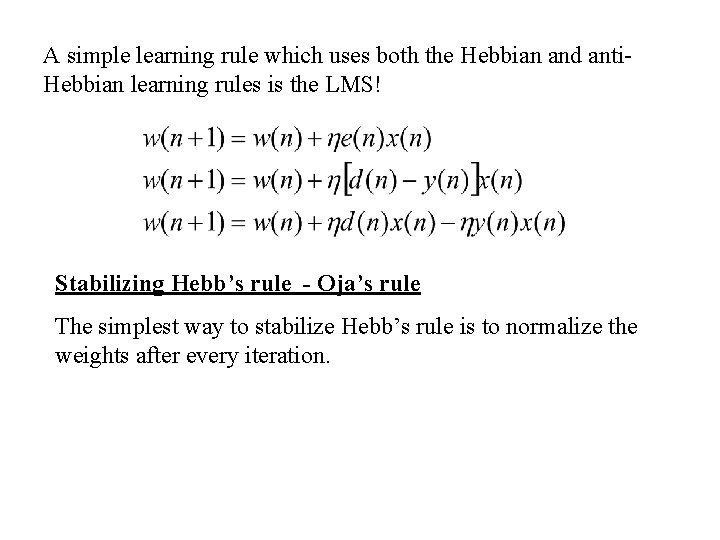
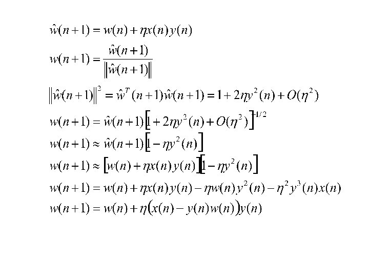
A simple learning rule which uses both the Hebbian and anti. Hebbian learning rules is the LMS! Stabilizing Hebb’s rule - Oja’s rule The simplest way to stabilize Hebb’s rule is to normalize the weights after every iteration.

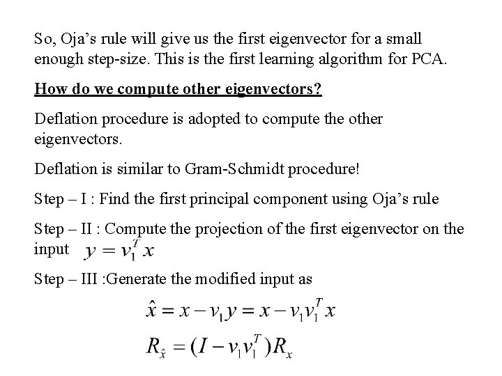
So, Oja’s rule will give us the first eigenvector for a small enough step-size. This is the first learning algorithm for PCA. How do we compute other eigenvectors? Deflation procedure is adopted to compute the other eigenvectors. Deflation is similar to Gram-Schmidt procedure! Step – I : Find the first principal component using Oja’s rule Step – II : Compute the projection of the first eigenvector on the input Step – III : Generate the modified input as

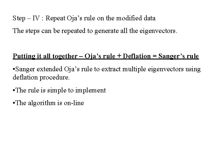
Step – IV : Repeat Oja’s rule on the modified data The steps can be repeated to generate all the eigenvectors. Putting it all together – Oja’s rule + Deflation = Sanger’s rule • Sanger extended Oja’s rule to extract multiple eigenvectors using deflation procedure. • The rule is simple to implement • The algorithm is on-line

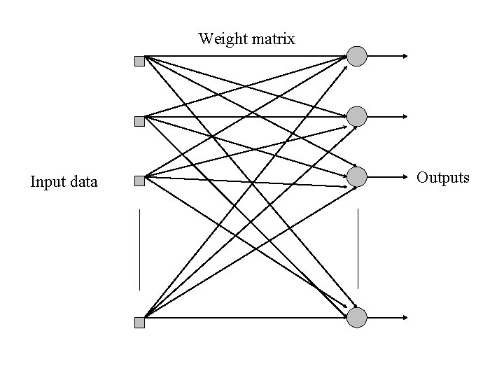
Weight matrix Input data Outputs

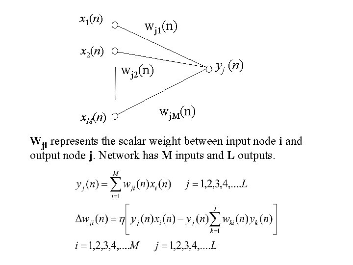
x 1(n) wj 1(n) x 2(n) yj (n) wj 2(n) x. M(n) wj. M(n) Wji represents the scalar weight between input node i and output node j. Network has M inputs and L outputs.