Adaptive Algorithms for Optimal Classification and Compression of

Adaptive Algorithms for Optimal Classification and Compression of Hyperspectral Images Tamal Bose* and Erzsébet Merényi# *Wireless@VT Bradley Dept. of Electrical and Computer Engineering Virginia Tech Electrical and Computer Engineering # Rice University

Outline u Motivation u Signal Processing System u Adaptive Differential Pulse Code Modulation (ADPCM) Scheme u Transform Scheme u Results u Conclusion

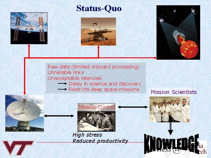
Status-Quo Raw data (limited onboard processing) Unreliable links Unacceptable latencies Delay in science and discovery Restricts deep space missions Mission Control High stress Reduced productivity Mission Scientists

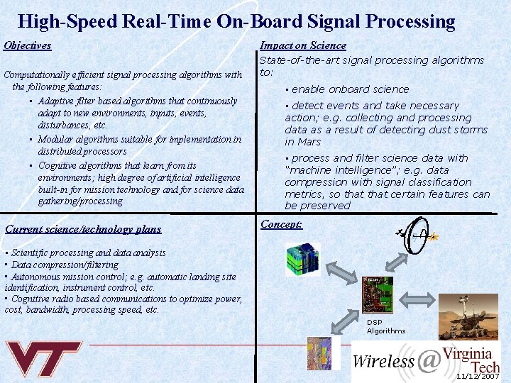
High-Speed Real-Time On-Board Signal Processing Objectives Computationally efficient signal processing algorithms with the following features: • Adaptive filter based algorithms that continuously adapt to new environments, inputs, events, disturbances, etc. • Modular algorithms suitable for implementation in distributed processors • Cognitive algorithms that learn from its environments; high degree of artificial intelligence built-in for mission technology and for science data gathering/processing Current science/technology plans Impact on Science State-of-the-art signal processing algorithms to: • enable onboard science • detect events and take necessary action; e. g. collecting and processing data as a result of detecting dust storms in Mars • process and filter science data with “machine intelligence”; e. g. data compression with signal classification metrics, so that certain features can be preserved Concept: • Scientific processing and data analysis • Data compression/filtering • Autonomous mission control; e. g. automatic landing site identification, instrument control, etc. • Cognitive radio based communications to optimize power, cost, bandwidth, processing speed, etc. DSP Algorithms 11/12/2007

Impact o Large body of knowledge developed for on-board processing. Two main classes (Filtering and Classification): n Adaptive filtering algorithms (EDS, FEDS, CG, and many variants) n Algorithms for 3 -D data de-noising, filtering, compression, and coding. n Algorithms for hyperspectral image clustering, classification, onboard science (Hyper. Eye) n Algorithms for joint classification and compression.

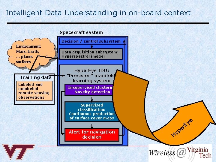
Intelligent Data Understanding in on-board context Spacecraft system Decision / control subsystem Environment: Mars, Earth, … planet surfaces Training data Labeled and unlabeled remote sensing observations Data acquisition subsystem: Hyperspectral imager Hyper. Eye IDU: “Precision” manifold learning system Unsupervised clustering Novelty detection Supervised classification: Continuous production of surface cover maps Alert for navigation decision e y E r H e p y

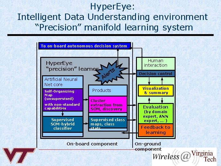
Hyper. Eye: Intelligent Data Understanding environment “Precision” manifold learning system To on-board autonomous decision system Hyper. Eye “precision” learner Artificial Neural Net core Self-Organizing Map (unsupervised) with non-standard capabilities Supervised SOM-hybrid classifier ts r e Al Products Cluster extraction from SOM, discovery Supervised class maps, class stats On-board component Human interaction Decision control Visualization & summary Evaluation (by domain expert, ANN expert, … ) Feedback to learning On-ground component

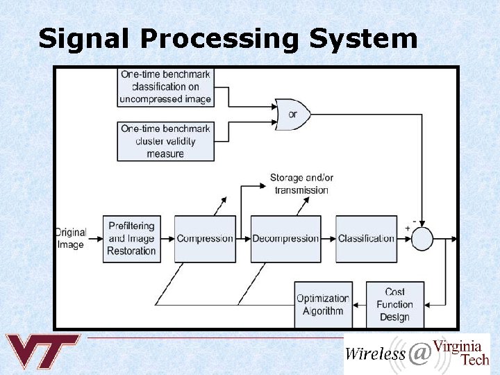
Specific Goals (this talk) o Maximize compression ratio with classification metrics o Minimize mean square error under some constraints o Minimize classification error

Signal Processing System

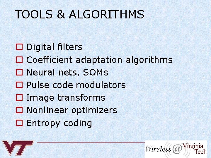
TOOLS & ALGORITHMS o o o o Digital filters Coefficient adaptation algorithms Neural nets, SOMs Pulse code modulators Image transforms Nonlinear optimizers Entropy coding

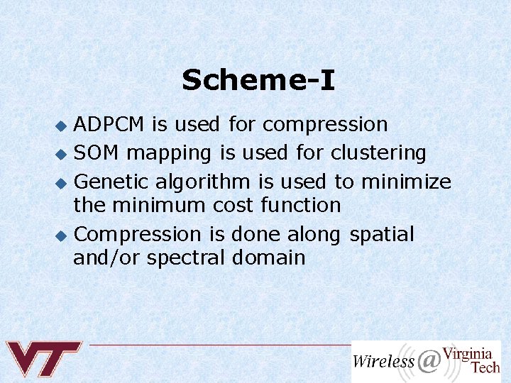
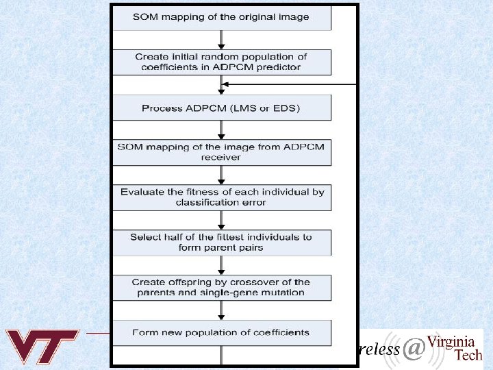
Scheme-I ADPCM is used for compression u SOM mapping is used for clustering u Genetic algorithm is used to minimize the minimum cost function u Compression is done along spatial and/or spectral domain u

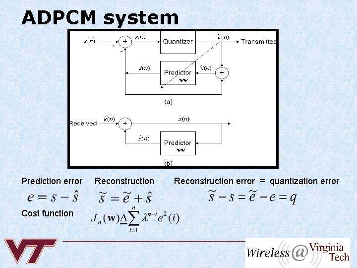
ADPCM system Prediction error Cost function Reconstruction error = quantization error

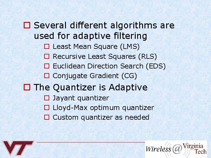
o Several different algorithms are used for adaptive filtering o o Least Mean Square (LMS) Recursive Least Squares (RLS) Euclidean Direction Search (EDS) Conjugate Gradient (CG) o The Quantizer is Adaptive o Jayant quantizer o Lloyd-Max optimum quantizer o Custom quantizer as needed

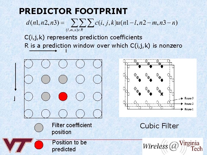
PREDICTOR FOOTPRINT C(i, j, k) represents prediction coefficients R is a prediction window over which C(i, j, k) is nonzero i j Filter coefficient position Position to be predicted Cubic Filter

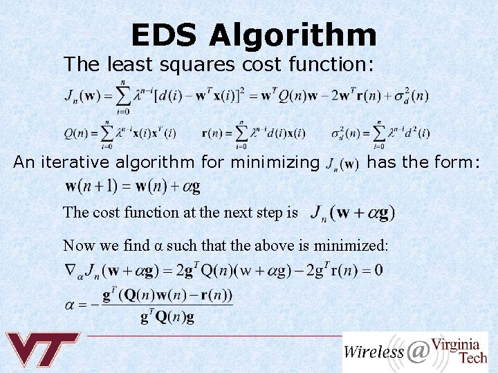
EDS Algorithm The least squares cost function: An iterative algorithm for minimizing has the form: The cost function at the next step is Now we find α such that the above is minimized:

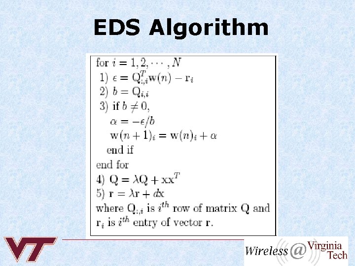
EDS Algorithm

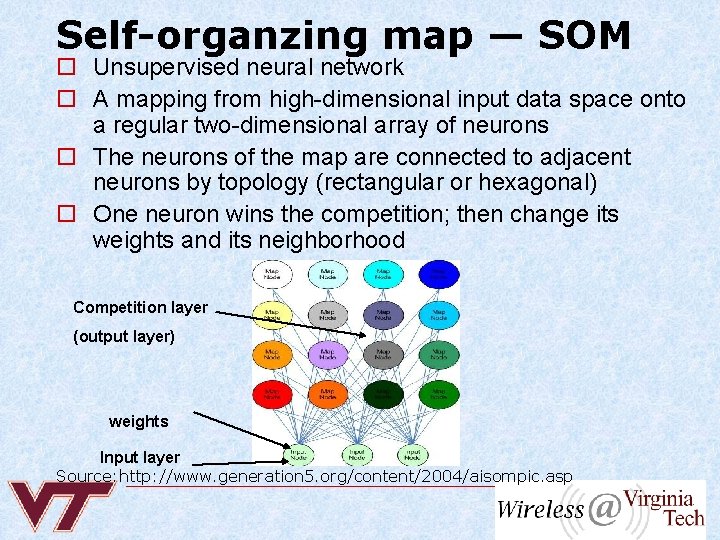
Self-organzing map — SOM o Unsupervised neural network o A mapping from high-dimensional input data space onto a regular two-dimensional array of neurons o The neurons of the map are connected to adjacent neurons by topology (rectangular or hexagonal) o One neuron wins the competition; then change its weights and its neighborhood Competition layer (output layer) weights Input layer Source: http: //www. generation 5. org/content/2004/aisompic. asp

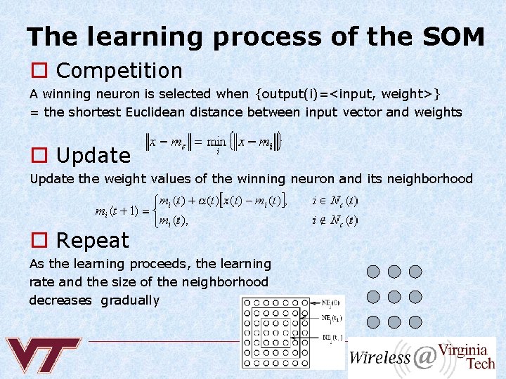
The learning process of the SOM o Competition A winning neuron is selected when {output(i)=<input, weight>} = the shortest Euclidean distance between input vector and weights o Update the weight values of the winning neuron and its neighborhood o Repeat As the learning proceeds, the learning rate and the size of the neighborhood decreases gradually

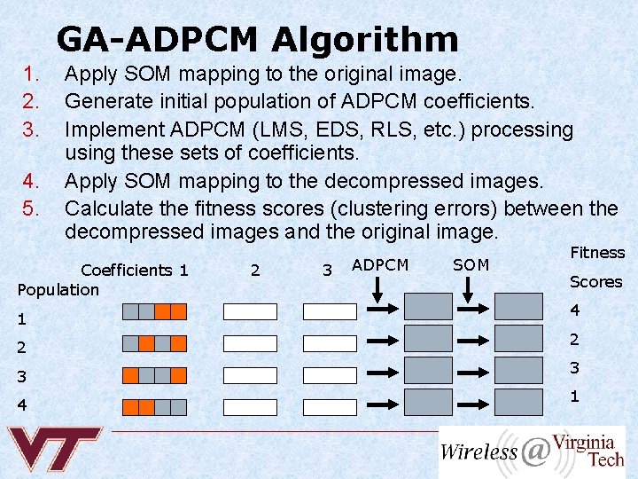
GA-ADPCM Algorithm 1. 2. 3. 4. 5. Apply SOM mapping to the original image. Generate initial population of ADPCM coefficients. Implement ADPCM (LMS, EDS, RLS, etc. ) processing using these sets of coefficients. Apply SOM mapping to the decompressed images. Calculate the fitness scores (clustering errors) between the decompressed images and the original image. Coefficients 1 Population 1 2 3 4 2 3 ADPCM SOM Fitness Scores 4 2 3 1

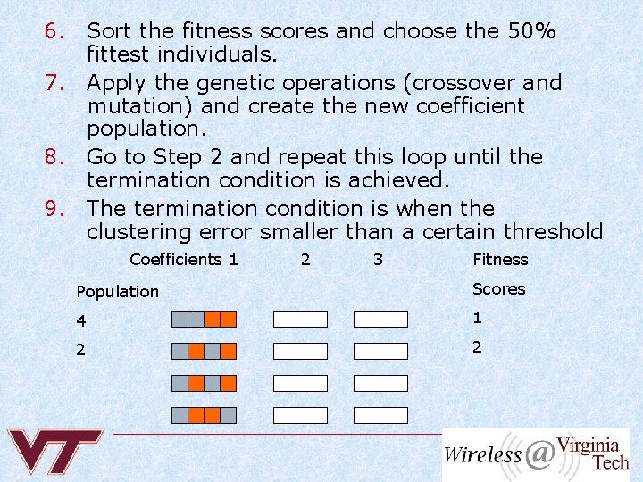
6. Sort the fitness scores and choose the 50% fittest individuals. 7. Apply the genetic operations (crossover and mutation) and create the new coefficient population. 8. Go to Step 2 and repeat this loop until the termination condition is achieved. 9. The termination condition is when the clustering error smaller than a certain threshold Coefficients 1 2 3 Fitness Population Scores 4 1 2 2

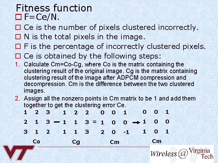
Fitness function o F=Ce/N. o o Ce is the number of pixels clustered incorrectly. N is the total pixels in the image. F is the percentage of incorrectly clustered pixels. Ce is obtained by the following steps: 1. Calculate Cm=Co-Cg, where Co is the matrix containing the clustering result of the original image. Cg is the matrix containing clustering result of the image after ADPCM compression and decompression. Cm is the difference between the two clustered images. 2. Assign all the nonzero points in Cm matrix to be 1 and add them together to get the clustering error Ce. 1 2 3 1 2 2 0 0 1 2 1 3 1 1 3 = 1 0 0 3 1 2 1 1 3 0 -1 1 0 1 Co Cg 2 Cm Cm

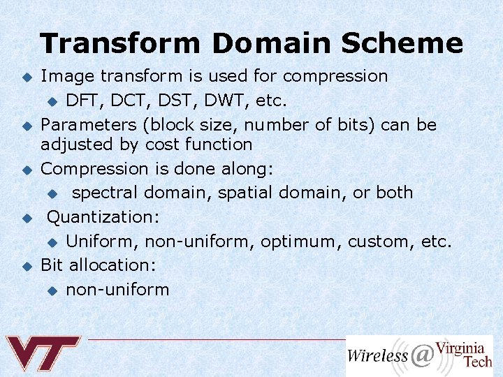
Transform Domain Scheme u u u Image transform is used for compression u DFT, DCT, DST, DWT, etc. Parameters (block size, number of bits) can be adjusted by cost function Compression is done along: u spectral domain, spatial domain, or both Quantization: u Uniform, non-uniform, optimum, custom, etc. Bit allocation: u non-uniform

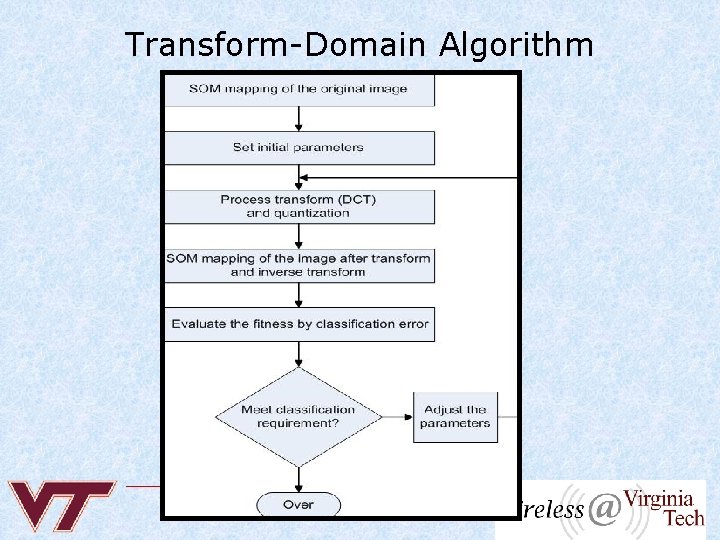
Transform-Domain Algorithm

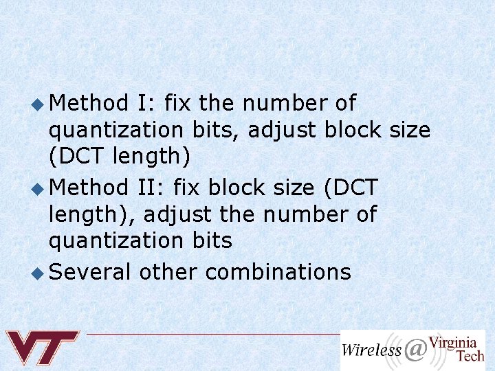
u Method I: fix the number of quantization bits, adjust block size (DCT length) u Method II: fix block size (DCT length), adjust the number of quantization bits u Several other combinations

Results

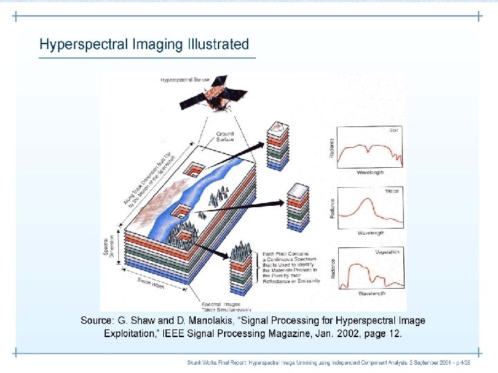
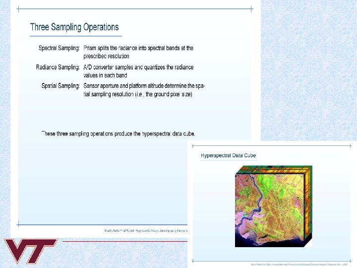
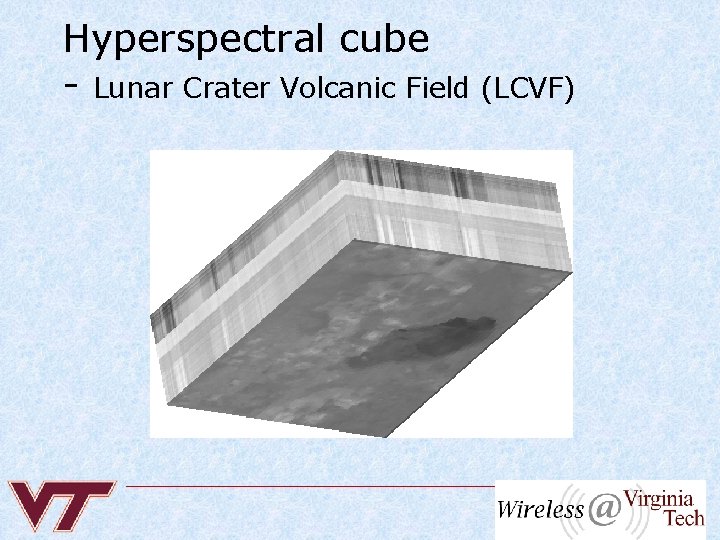
Hyperspectral cube - Lunar Crater Volcanic Field (LCVF)

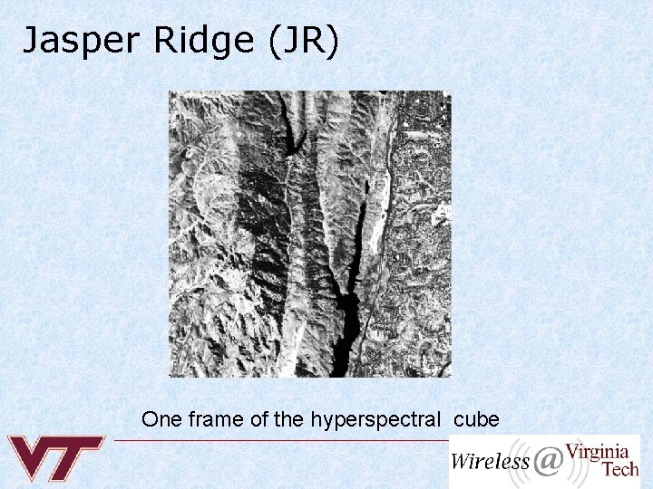
Jasper Ridge (JR) One frame of the hyperspectral cube

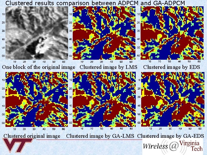
Clustered results comparison between ADPCM and GA-ADPCM One block of the original image Clustered image by LMS Clustered original image Clustered image by EDS Clustered image by GA-LMS Clustered image by GA-EDS

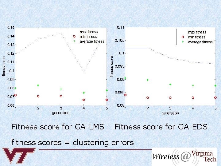
Fitness score for GA-LMS Fitness score for GA-EDS fitness scores = clustering errors

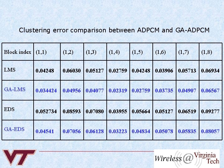
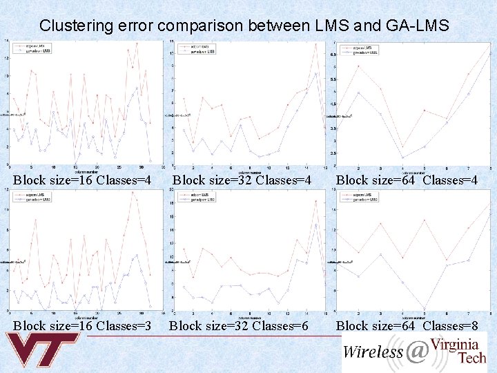
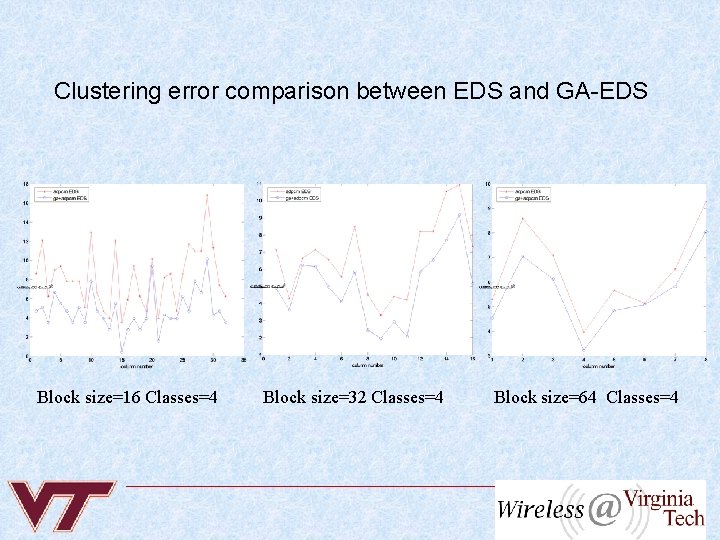
Clustering error comparison between ADPCM and GA-ADPCM Block index (1, 1) (1, 2) (1, 3) (1, 4) (1, 5) (1, 6) (1, 7) (1, 8) LMS 0. 04248 0. 06030 0. 05127 0. 02759 0. 04248 0. 03906 0. 05713 0. 06934 GA-LMS 0. 034424 0. 04956 0. 04077 0. 02319 0. 02759 0. 03735 0. 04907 0. 06567 EDS 0. 052734 0. 08593 0. 07080 0. 03955 0. 05664 0. 05127 0. 06519 0. 09277 GA-EDS 0. 04541 0. 07056 0. 06128 0. 03223 0. 04834 0. 05078 0. 05835 0. 08057

Clustering error comparison between LMS and GA-LMS Block size=16 Classes=4 Block size=32 Classes=4 Block size=64 Classes=4 Block size=16 Classes=3 Block size=32 Classes=6 Block size=64 Classes=8

Clustering error comparison between EDS and GA-EDS Block size=16 Classes=4 Block size=32 Classes=4 Block size=64 Classes=4

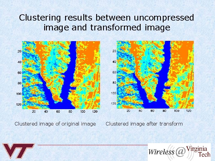
Clustering results between uncompressed image and transformed image Clustered image of original image Clustered image after transform

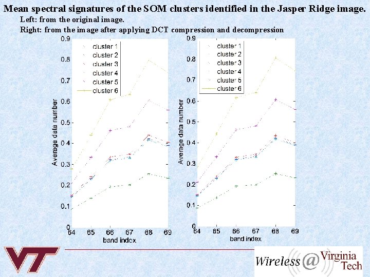
Mean spectral signatures of the SOM clusters identified in the Jasper Ridge image. Left: from the original image. Right: from the image after applying DCT compression and decompression

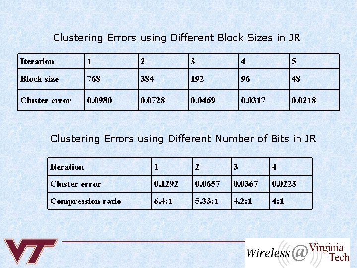
Clustering Errors using Different Block Sizes in JR Iteration 1 2 3 4 5 Block size 768 384 192 96 48 Cluster error 0. 0980 0. 0728 0. 0469 0. 0317 0. 0218 Clustering Errors using Different Number of Bits in JR Iteration 1 2 3 4 Cluster error 0. 1292 0. 0657 0. 0367 0. 0223 Compression ratio 6. 4: 1 5. 33: 1 4. 2: 1 4: 1

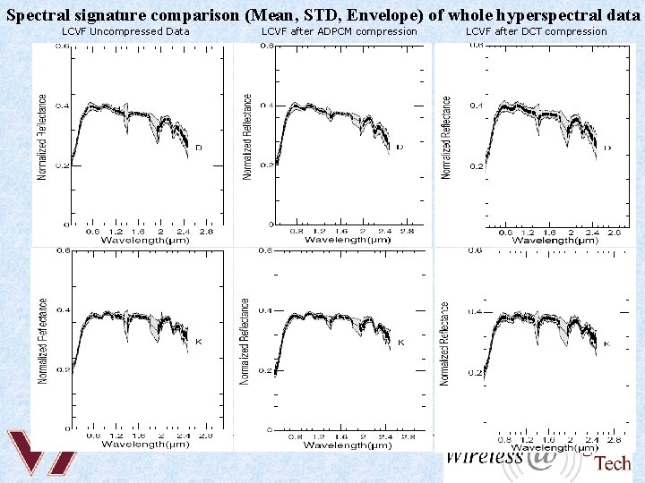
Spectral signature comparison (Mean, STD, Envelope) of whole hyperspectral data LCVF Uncompressed Data LCVF after ADPCM compression LCVF after DCT compression

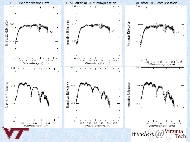
LCVF Uncompressed Data LCVF after ADPCM compression LCVF after DCT compression

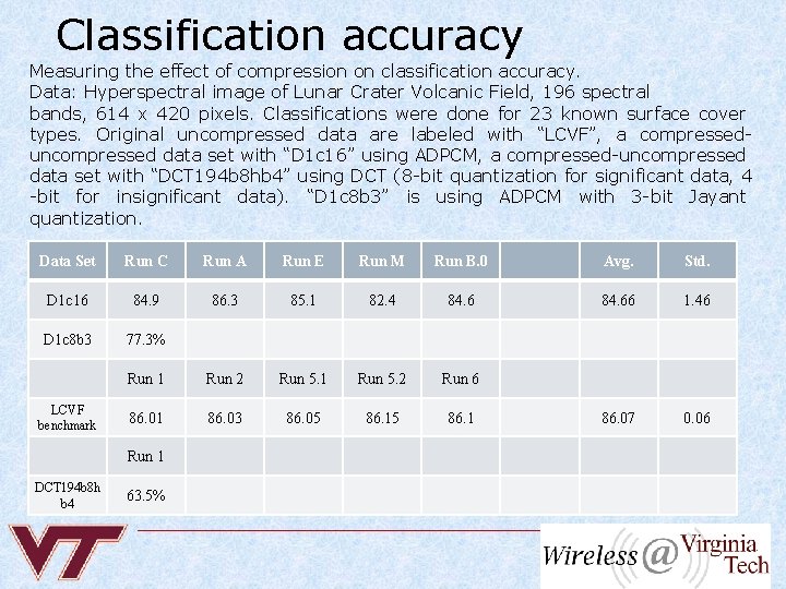
Classification accuracy Measuring the effect of compression on classification accuracy. Data: Hyperspectral image of Lunar Crater Volcanic Field, 196 spectral bands, 614 x 420 pixels. Classifications were done for 23 known surface cover types. Original uncompressed data are labeled with “LCVF”, a compresseduncompressed data set with “D 1 c 16” using ADPCM, a compressed-uncompressed data set with “DCT 194 b 8 hb 4” using DCT (8 -bit quantization for significant data, 4 -bit for insignificant data). “D 1 c 8 b 3” is using ADPCM with 3 -bit Jayant quantization. Data Set Run C Run A Run E Run M Run B. 0 Avg. Std. D 1 c 16 84. 9 86. 3 85. 1 82. 4 84. 66 1. 46 D 1 c 8 b 3 77. 3% Run 1 Run 2 Run 5. 1 Run 5. 2 Run 6 86. 01 86. 03 86. 05 86. 1 86. 07 0. 06 LCVF benchmark Run 1 DCT 194 b 8 h b 4 63. 5%

Conclusion New algorithms have been developed and implemented that use the concept of classification metric driven compression o GA-ADPCM algorithm was simulated: n Optimized the adaptive filter in an ADPCM using GA n Reduced clustering error n Drawback – increased computational cost o Feedback-Transform algorithm was simulated: n Select the optimal block size (DCT length) and number of quantization bits to achieve a balance between a low clustering error, and computational complexity, and memory usage n Compression along spectral domain preserves the spectral signatures of the clusters o Results using the above algorithms are promising o

Acknowledgments o Graduate students: n n n Mike Larsen (USU) Kay Thamvichai (USU) Mike Mendenhall (Rice) Li Ling (Rice) Bei Xei (VT) B. Ramkumar (VT) o NASA AISR Program