Actors in SALSA and Erlang PDCS 9 CPE

Actors in SALSA and Erlang (PDCS 9, CPE 5*) Support for actor model in SALSA and Erlang Carlos Varela Rennselaer Polytechnic Institute October 9, 2015 * Concurrent Programming in Erlang, by J. Armstrong, R. Virding, C. Wikström, M. Williams C. Varela 1

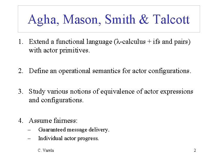
Agha, Mason, Smith & Talcott 1. Extend a functional language (λ-calculus + ifs and pairs) with actor primitives. 2. Define an operational semantics for actor configurations. 3. Study various notions of equivalence of actor expressions and configurations. 4. Assume fairness: – – Guaranteed message delivery. Individual actor progress. C. Varela 2

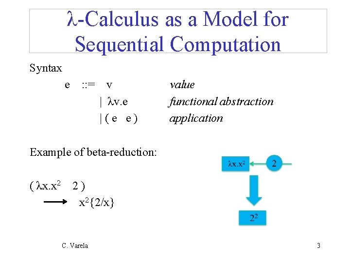
λ-Calculus as a Model for Sequential Computation Syntax e : : = v | λv. e |(e e) value functional abstraction application Example of beta-reduction: ( λx. x 2 2 ) x 2{2/x} C. Varela 3

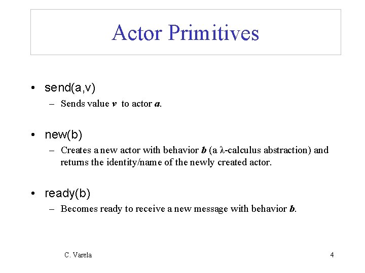
Actor Primitives • send(a, v) – Sends value v to actor a. • new(b) – Creates a new actor with behavior b (a λ-calculus abstraction) and returns the identity/name of the newly created actor. • ready(b) – Becomes ready to receive a new message with behavior b. C. Varela 4

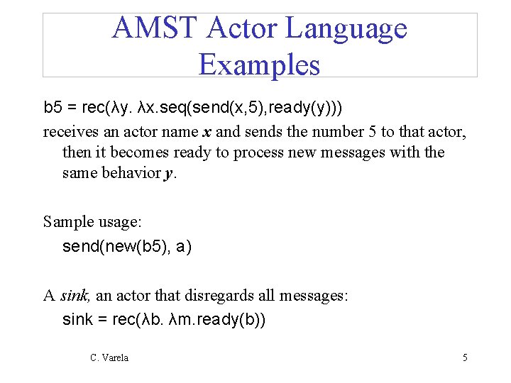
AMST Actor Language Examples b 5 = rec(λy. λx. seq(send(x, 5), ready(y))) receives an actor name x and sends the number 5 to that actor, then it becomes ready to process new messages with the same behavior y. Sample usage: send(new(b 5), a) A sink, an actor that disregards all messages: sink = rec(λb. λm. ready(b)) C. Varela 5

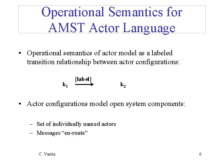
Operational Semantics for AMST Actor Language • Operational semantics of actor model as a labeled transition relationship between actor configurations: k 1 [label] k 2 • Actor configurations model open system components: – Set of individually named actors – Messages “en-route” C. Varela 6

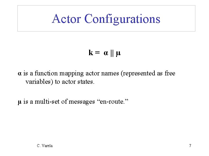
Actor Configurations k = α || µ α is a function mapping actor names (represented as free variables) to actor states. µ is a multi-set of messages “en-route. ” C. Varela 7

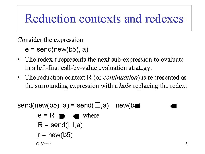
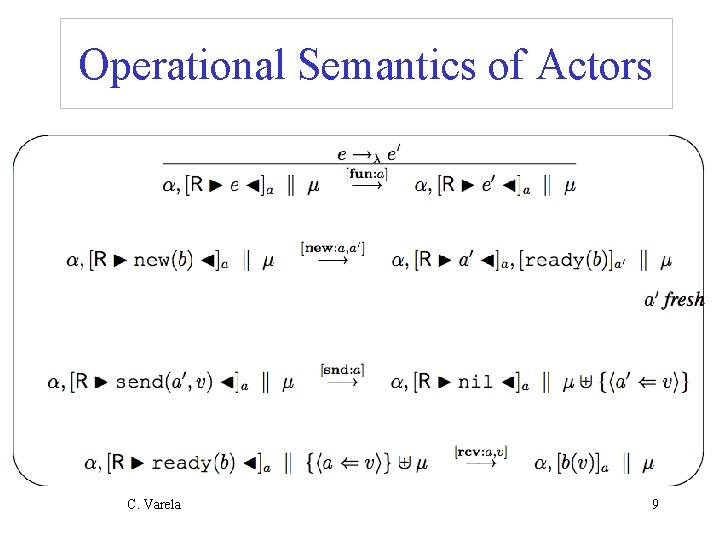
Reduction contexts and redexes Consider the expression: e = send(new(b 5), a) • The redex r represents the next sub-expression to evaluate in a left-first call-by-value evaluation strategy. • The reduction context R (or continuation) is represented as the surrounding expression with a hole replacing the redex. send(new(b 5), a) = send(☐, a) e=R r where R = send(☐, a) r = new(b 5) C. Varela new(b 5) 8

Operational Semantics of Actors C. Varela 9

Operational semantics example (1) k 0 = [send(☐, a) new(b 5) ]a || {} k 1 = [send(b, a)]a, [ready(b 5)]b || {} [new: a, b] k 0 k 1 k 2 = [nil]a, [ready(b 5)]b || {< b <= a >} [snd: a] k 1 C. Varela k 2 10

Operational semantics example (2) k 2 = [nil]a, [ready(b 5)]b || {< b <= a >} k 3 = [nil]a, [rec(λy. λx. seq(send(x, 5), ready(y)))(a)]b || {} [rcv: b, a] k 2 k 3 k 4 = [nil]a, [seq(send(a, 5), ready(b 5)))]b || {} [fun: b] k 3 C. Varela k 4 11

Operational semantics example (3) k 4 = [nil]a, [seq(☐, ready(b 5)) send(a, 5) ]b || {} [snd: a, 5] k 4 k 5 = [nil]a, [seq(nil, ready(b 5))]b || {< a <= 5 >} C. Varela 12

Operational semantics example (4) k 5 = [nil]a, [seq(nil, ready(b 5))]b || {< a <= 5 >} k 6 = [nil]a, [ready(b 5)]b || {< a <= 5 >} [fun: b] k 5 C. Varela k 6 13

Semantics example summary k 0 = [send(new(b 5), a)]a || {} k 6 = [nil]a, [ready(b 5)]b || {< a <= 5 >} k 0 k 4 [new: a, b] [snd: a] k 1 [snd: a, 5] [fun: b] k 5 C. Varela [rcv: b, a] k 2 k 6 [fun: b] k 3 k 4 This sequence of (labeled) transitions from k 0 to k 6 is called a computation sequence. 14

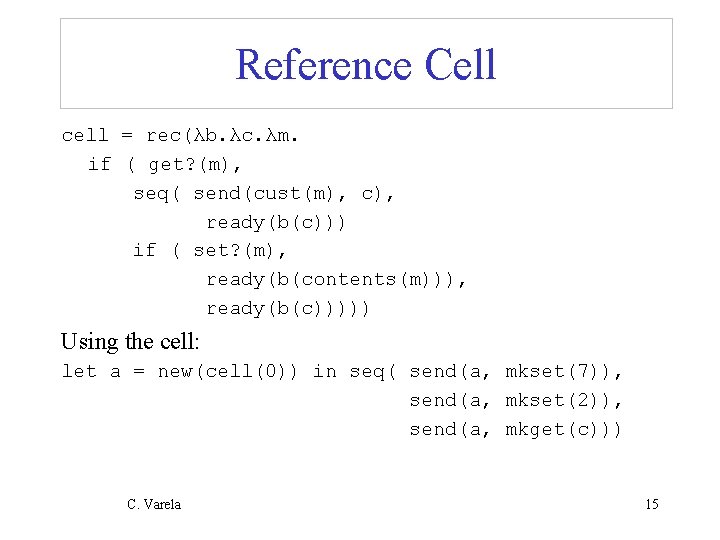
Reference Cell cell = rec(λb. λc. λm. if ( get? (m), seq( send(cust(m), c), ready(b(c))) if ( set? (m), ready(b(contents(m))), ready(b(c))))) Using the cell: let a = new(cell(0)) in seq( send(a, mkset(7)), send(a, mkset(2)), send(a, mkget(c))) C. Varela 15

Asynchronous communication k 0 = [ready(cell(0))]a || {<a<=s(7)>, <a<=s(2)>, <a<=g(c)>} Three receive transitions are enabled at k 0 k 0 [rcv: a, s(7)] [rcv: a, s(2)] [rcv: a, g(c)] C. Varela k 1’ k 1” Multiple enabled transitions can lead to nondeterministic behavior The set of all computations sequences from k 0 is called the computation tree τ(k 0). 16

Nondeterministic behavior (1) k 0 = [ready(cell(0))]a || {<a<=s(7)>, <a<=s(2)>, <a<=g(c)>} k 1 * [ready(cell(7))]a || {<a<=s(2)>, <a<=g(c)>} Customer c will get 2 or 7. k 1’ * [ready(cell(2))]a || {<a<=s(7)>, <a<=g(c)>} Customer c will get 0. k 1” * [ready(cell(0))]a || {<a<=s(7)>, <a<=s(2)>, <c<=0>} C. Varela 17

Nondeterministic behavior (2) k 0 = [ready(cell(0))]a || {<a<=s(7)>, <a<=s(2)>, <a<=g(c)>} Order of three receive transitions determines final state, e. g. : k 0 [rcv: a, g(c)] [rcv: a, s(7)] k 1 * k 2 [rcv: a, s(2)] * k 3 kf = [ready(cell(2))]a || {<c<=0>} Final cell state is 2. C. Varela 18

Nondeterministic behavior (3) k 0 = [ready(cell(0))]a || {<a<=s(7)>, <a<=s(2)>, <a<=g(c)>} Order of three receive transitions determines final state, e. g. : k 0 [rcv: a, s(2)] [rcv: a, g(c)] k 1 * k 2 [rcv: a, s(7)] * k 3 kf = [ready(cell(7))]a || {<c<=2>} Final cell state is 7. C. Varela 19

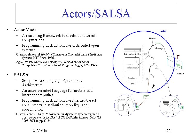
Actors/SALSA • Actor Model – A reasoning framework to model concurrent computations – Programming abstractions for distributed open systems G. Agha, Actors: A Model of Concurrent Computation in Distributed Systems. MIT Press, 1986. Agha, Mason, Smith and Talcott, “A Foundation for Actor Computation”, J. of Functional Programming, 7, 1 -72, 1997. • SALSA – Simple Actor Language System and Architecture – An actor-oriented language for mobile and internet computing – Programming abstractions for internet-based concurrency, distribution, mobility, and coordination C. Varela and G. Agha, “Programming dynamically reconfigurable open systems with SALSA”, ACM SIGPLAN Notices, OOPSLA 2001, 36(12), pp 20 -34. C. Varela 20

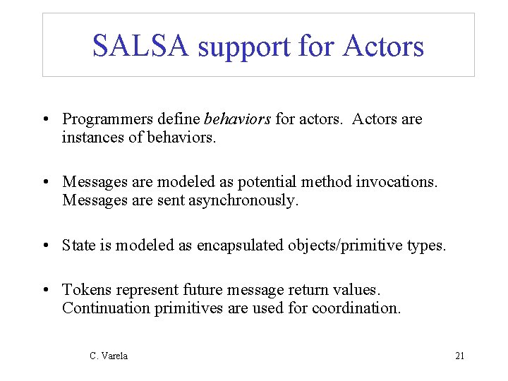
SALSA support for Actors • Programmers define behaviors for actors. Actors are instances of behaviors. • Messages are modeled as potential method invocations. Messages are sent asynchronously. • State is modeled as encapsulated objects/primitive types. • Tokens represent future message return values. Continuation primitives are used for coordination. C. Varela 21

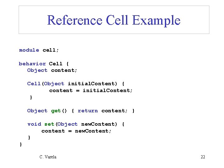
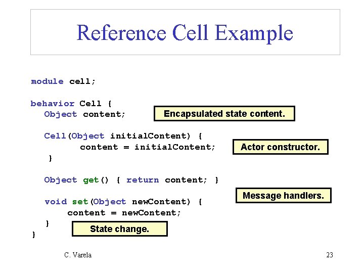
Reference Cell Example module cell; behavior Cell { Object content; Cell(Object initial. Content) { content = initial. Content; } Object get() { return content; } void set(Object new. Content) { content = new. Content; } } C. Varela 22

Reference Cell Example module cell; behavior Cell { Object content; Encapsulated state content. Cell(Object initial. Content) { content = initial. Content; } Actor constructor. Object get() { return content; } } void set(Object new. Content) { content = new. Content; } State change. C. Varela Message handlers. 23

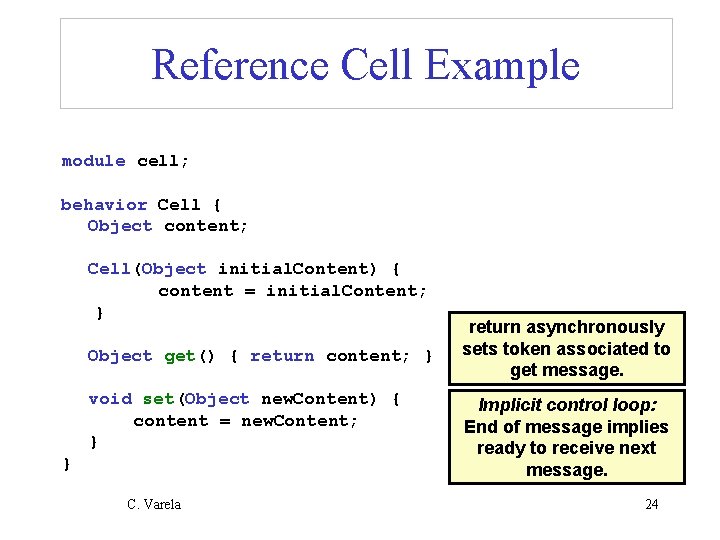
Reference Cell Example module cell; behavior Cell { Object content; Cell(Object initial. Content) { content = initial. Content; } Object get() { return content; } void set(Object new. Content) { content = new. Content; } } C. Varela return asynchronously sets token associated to get message. Implicit control loop: End of message implies ready to receive next message. 24

Cell Tester Example module cell; behavior Cell. Tester { void act( String[] args ) { Cell c = new Cell(0); c <- set(2); c <- set(7); token t = c <- get(); standard. Output <- println( t ); } } C. Varela 25

Cell Tester Example module cell; behavior Cell. Tester { void act( String[] args ) { Actor creation (new) Cell c = new Cell(0); c <- set(2); c <- set(7); Message passing token t = c <- get(); standard. Output <- println( t ); } (<-) println message can only be processed when token t from c’s get() message handler has been produced. } C. Varela 26

Cell Tester Example module cell; behavior Cell. Tester { void act( String[] args ) { Cell c = new Cell(0); c <- set(2); c <- set(7); token t = c <- get(); standard. Output <- println( t ); } } C. Varela All message passing is asynchronous. println message is called partial until token t is produced. Only full messages (with no pending tokens) are delivered to actors. 27

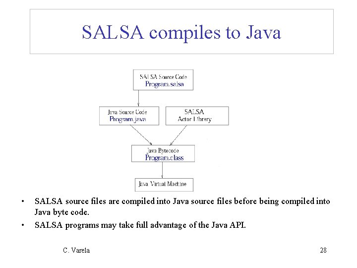
SALSA compiles to Java • • SALSA source files are compiled into Java source files before being compiled into Java byte code. SALSA programs may take full advantage of the Java API. C. Varela 28

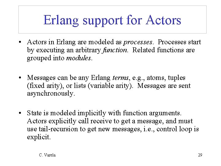
Erlang support for Actors • Actors in Erlang are modeled as processes. Processes start by executing an arbitrary function. Related functions are grouped into modules. • Messages can be any Erlang terms, e. g. , atoms, tuples (fixed arity), or lists (variable arity). Messages are sent asynchronously. • State is modeled implicitly with function arguments. Actors explicitly call receive to get a message, and must use tail-recursion to get new messages, i. e. , control loop is explicit. C. Varela 29

Reference Cell in Erlang -module(cell). -export([cell/1]). cell(Content) -> receive {set, New. Content} -> cell(New. Content); {get, Customer} -> Customer ! Content, cell(Content) end. C. Varela 30

Reference Cell in Erlang -module(cell). -export([cell/1]). Encapsulated state Content. cell(Content) -> receive {set, New. Content} -> cell(New. Content); State Message {get, Customer} -> Customer ! Content, handlers cell(Content) end. change. Explicit control loop: Actions at the end of a message need to include tail-recursive function call. Otherwise actor (process) terminates. C. Varela 31

Reference Cell in Erlang -module(cell). -export([cell/1]). Content is an argument to the cell function. cell(Content) -> receive {set, New. Content} -> cell(New. Content); {get, Customer} -> Customer ! Content, cell(Content) end. {set, New. Content} is a tuple pattern. set is an atom. New. Content is a variable. Messages are checked one by one, and for each message, first pattern that applies gets its actions (after ->) executed. If no pattern matches, messages remain in actor’s mailbox. C. Varela 32

Cell Tester in Erlang -module(cell. Tester). -export([main/0]). main() -> C = spawn(cell, [0]), C!{set, 2}, C!{set, 7}, C!{get, self()}, receive Value -> io: format("~w~n”, [Value]) end. C. Varela 33

Cell Tester in Erlang -module(cell. Tester). -export([main/0]). main() -> C = spawn(cell, [0]), Actor creation (spawn) C!{set, 2}, Message passing (!) C!{set, 7}, C!{get, self()}, receive waits until a Value -> message is available. io: format("~w~n”, [Value]) end. C. Varela 34

Cell Tester in Erlang -module(cell. Tester). -export([main/0]). [0] is a list with the arguments to the module’s function. General form: main() -> C = spawn(cell, [0]), C!{set, 2}, C!{set, 7}, spawn(module, function, C!{get, self()}, arguments) receive Value -> io: format("~w~n", [Value]) end. Function calls take the form: module: function(args) C. Varela self() is a built-in function (BIF) that returns the process id of the current process. 35

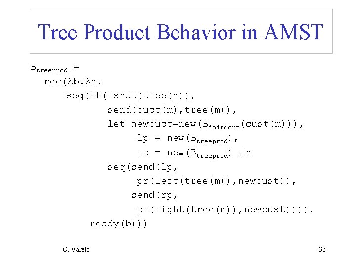
Tree Product Behavior in AMST Btreeprod = rec(λb. λm. seq(if(isnat(tree(m)), send(cust(m), tree(m)), let newcust=new(Bjoincont(cust(m))), lp = new(Btreeprod), rp = new(Btreeprod) in seq(send(lp, pr(left(tree(m)), newcust)), send(rp, pr(right(tree(m)), newcust)))), ready(b))) C. Varela 36

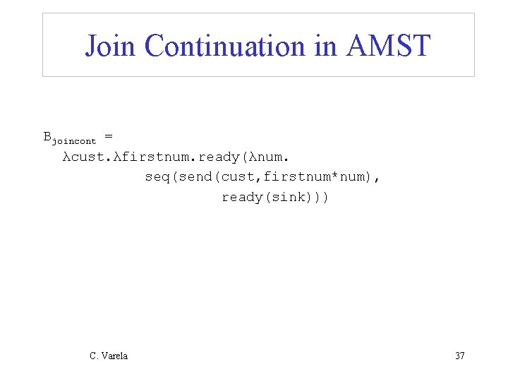
Join Continuation in AMST Bjoincont = λcust. λfirstnum. ready(λnum. seq(send(cust, firstnum*num), ready(sink))) C. Varela 37

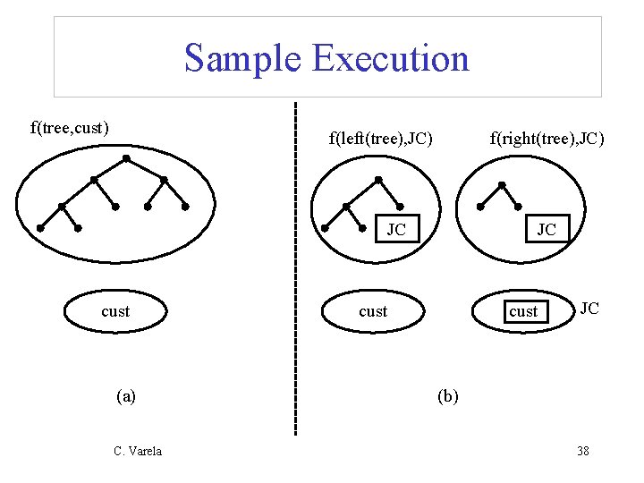
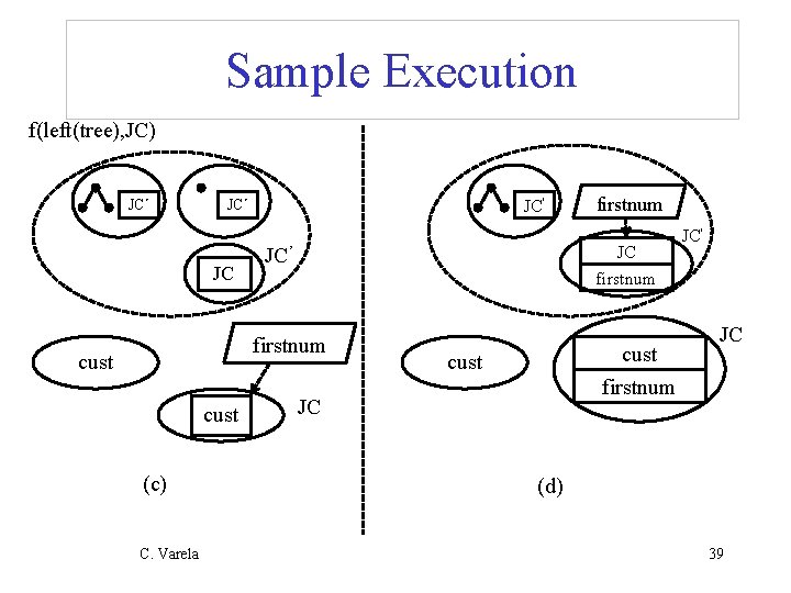
Sample Execution f(tree, cust) f(left(tree), JC) f(right(tree), JC) JC cust (a) C. Varela JC cust JC (b) 38

Sample Execution f(left(tree), JC) JC’ JC JC' JC firstnum JC’ firstnum cust (c) C. Varela firstnum cust JC JC' JC (d) 39

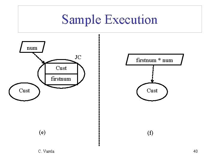
Sample Execution num JC firstnum * num Cust firstnum Cust (e) C. Varela (f) 40

Tree Product Behavior in Erlang -module(treeprod). -export([treeprod/0, join/1]). treeprod() -> receive {{Left, Right}, Customer} -> New. Cust = spawn(treeprod, join, [Customer]), LP = spawn(treeprod, []), RP = spawn(treeprod, []), LP!{Left, New. Cust}, RP!{Right, New. Cust}; {Number, Customer} -> Customer ! Number end, treeprod(). join(Customer) -> receive V 1 -> receive V 2 -> Customer ! V 1*V 2 end. C. Varela 41

Tree Product Sample Execution 2> TP = spawn(treeprod, []). <0. 40. 0> 3> TP ! {{{{5, 6}, 2}, {3, 4}}, self()}. {{{{5, 6}, 2}, {3, 4}}, <0. 33. 0>} 4> flush(). Shell got 720 ok 5> C. Varela 42

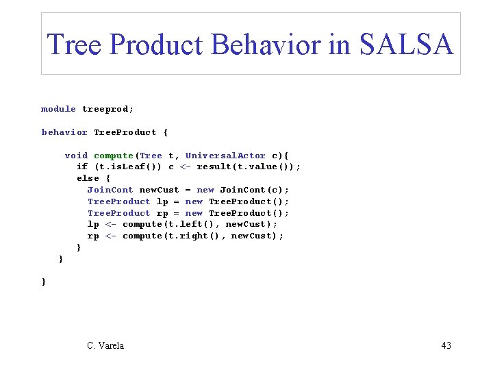
Tree Product Behavior in SALSA module treeprod; behavior Tree. Product { void compute(Tree t, Universal. Actor c){ if (t. is. Leaf()) c <- result(t. value()); else { Join. Cont new. Cust = new Join. Cont(c); Tree. Product lp = new Tree. Product(); Tree. Product rp = new Tree. Product(); lp <- compute(t. left(), new. Cust); rp <- compute(t. right(), new. Cust); } } } C. Varela 43

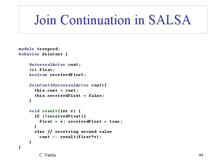
Join Continuation in SALSA module treeprod; behavior Join. Cont { Universal. Actor cust; int first; boolean received. First; Join. Cont(Universal. Actor cust){ this. cust = cust; this. received. First = false; } void result(int v) { if (!received. First){ first = v; received. First = true; } else // receiving second value cust <- result(first*v); } } C. Varela 44

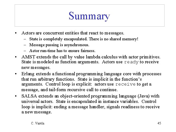
Summary • Actors are concurrent entities that react to messages. – State is completely encapsulated. There is no shared memory! – Message passing is asynchronous. – Actor run-time has to ensure fairness. • AMST extends the call by value lambda calculus with actor primitives. State is modeled as function arguments. Actors use ready to receive new messages. • Erlang extends a functional programming language core with processes that run arbitrary functions. State is implicit in the function’s arguments. Control loop is explicit: actors use receive to get a message, and tail-form recursive call to continue. • SALSA extends an object-oriented programming language (Java) with universal actors. State is encapsulated in instance variables. Control loop is implicit: ending a message handler, signals readiness to receive a new message. C. Varela 45

Exercises 41. Define pairing primitives (pr, 1 st, 2 nd) in the pure lambda calculus. 42. PDCS Exercise 4. 6. 1 (page 77). 43. Modify the treeprod behavior in Erlang to reuse the tree productor actor to compute the product of the left subtree. (See PDCS page 63 for the corresponding tprod 2 behavior in AMST. ) 44. PDCS Exercise 9. 6. 1 (page 203). 45. Create a concurrent fibonacci behavior in Erlang using join continuations. C. Varela 46