Active Learning Learning from Examples Passive learning l

Active Learning

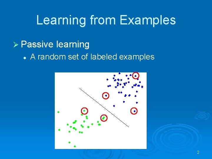
Learning from Examples Ø Passive learning l A random set of labeled examples 2

Active Learning Ø Active learning l The leaner chooses the specific examples to be labeled The learner works harder, in order to use fewer examples 3

Membership Queries Ø The learner constructs the examples from basic units Ø Examples of problems that are only solvable under this setting (finite automata) Problem: might get to irrelevant regions of the input space 4

Selective Sampling Ø Available are 2 oracles: l l Sample – returning unlabeled queries according to the input distribution Label – given an unlabeled example, returns its label Ø Query filtering – From the set of unlabeled examples, choose the most informative, and query for their label. 5

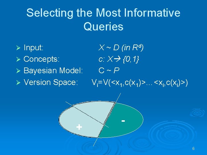
Selecting the Most Informative Queries Input: Ø Concepts: Ø Bayesian Model: Ø Version Space: Ø X ~ D (in Rd) c: X {0, 1} C~P Vi=V(<x 1, c(x 1)>…<xi, c(xi)>) + + 6

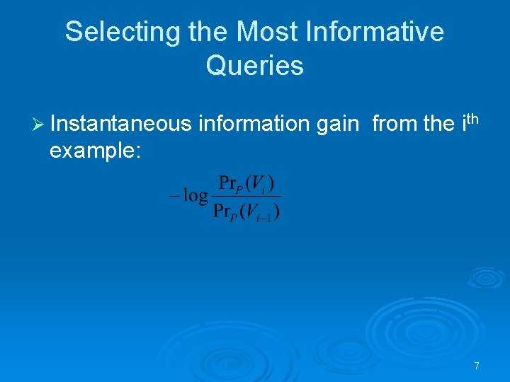
Selecting the Most Informative Queries Ø Instantaneous information gain from the ith example: 7

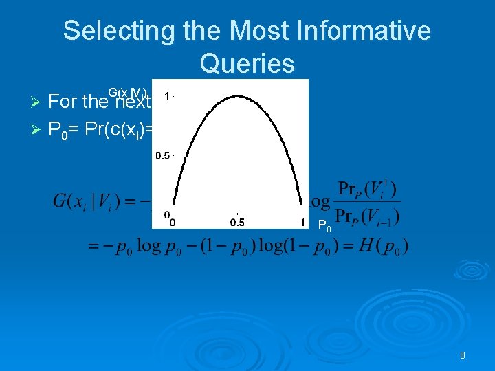
Selecting the Most Informative Queries G(xi|Vi) For the next example xi: Ø P 0= Pr(c(xi)==0) Ø P 0 8

Example Ø X = [0, 1] Ø W ~ U; Ø Vi=[the max X value labeled with 0, the min X value labeled with 1] - - - + + + 9

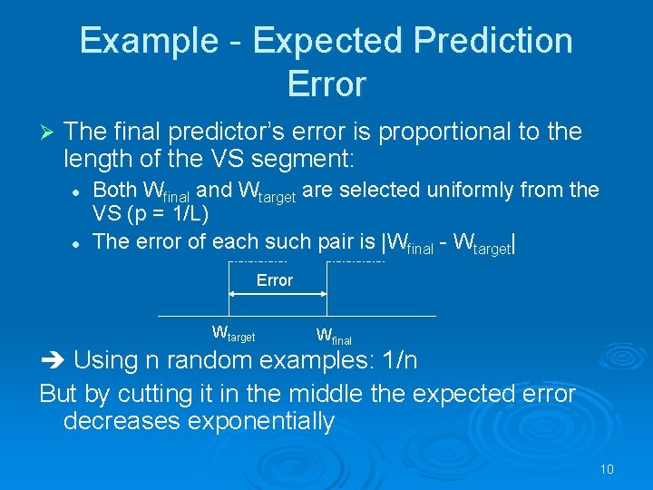
Example - Expected Prediction Error Ø The final predictor’s error is proportional to the length of the VS segment: l l Both Wfinal and Wtarget are selected uniformly from the VS (p = 1/L) The error of each such pair is |Wfinal - Wtarget| Error Wtarget Wfinal Using n random examples: 1/n But by cutting it in the middle the expected error decreases exponentially 10

Query by Committee (Seung, Opper & Sompolinsky 1992; Freund, Seung, Shamir & Tishby) Ø Uses oracles: l Gibbs(V, x) • h randp(V) • Return h(x) l l Sample Lable(x) 11

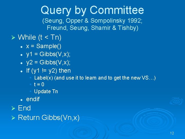
Query by Committee (Seung, Opper & Sompolinsky 1992; Freund, Seung, Shamir & Tishby) Ø While (t < Tn) l l x = Sample() y 1 = Gibbs(V, x); y 2 = Gibbs(V, x); If (y 1 != y 2) then • • • l Label(x) (and use it to learn and to get the new VS…) t=0 Update Tn endif End Ø Return Gibbs(Vn, x) Ø 12

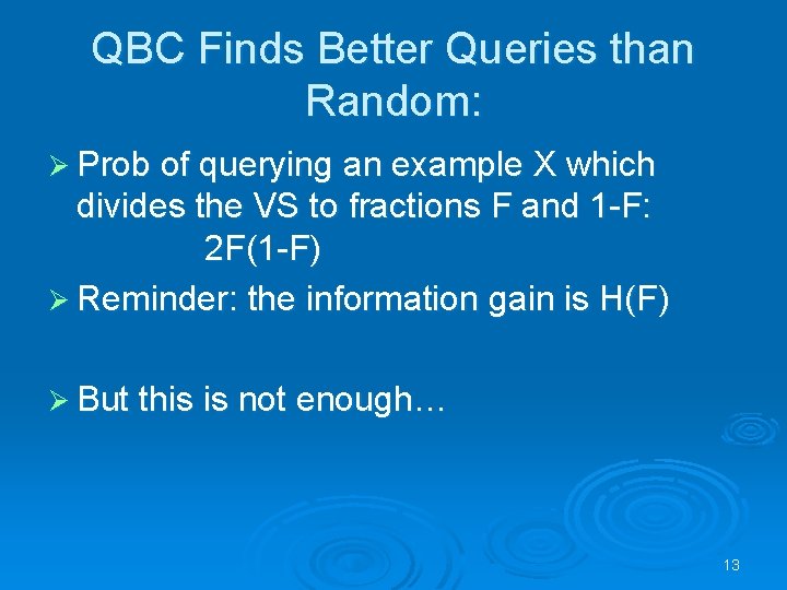
QBC Finds Better Queries than Random: Ø Prob of querying an example X which divides the VS to fractions F and 1 -F: 2 F(1 -F) Ø Reminder: the information gain is H(F) Ø But this is not enough… 13

Example Ø W is in [0, 1]2 Ø X is a line parallel to one of the axes Ø The error is proportional to the perimeter of the VS rectangle 14

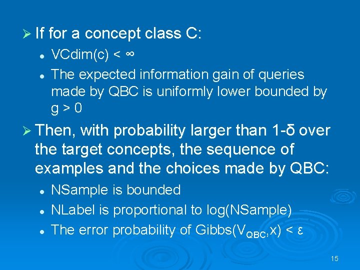
Ø If for a concept class C: l l VCdim(c) < ∞ The expected information gain of queries made by QBC is uniformly lower bounded by g>0 Ø Then, with probability larger than 1 -δ over the target concepts, the sequence of examples and the choices made by QBC: l l l NSample is bounded NLabel is proportional to log(NSample) The error probability of Gibbs(VQBC, x) < ε 15

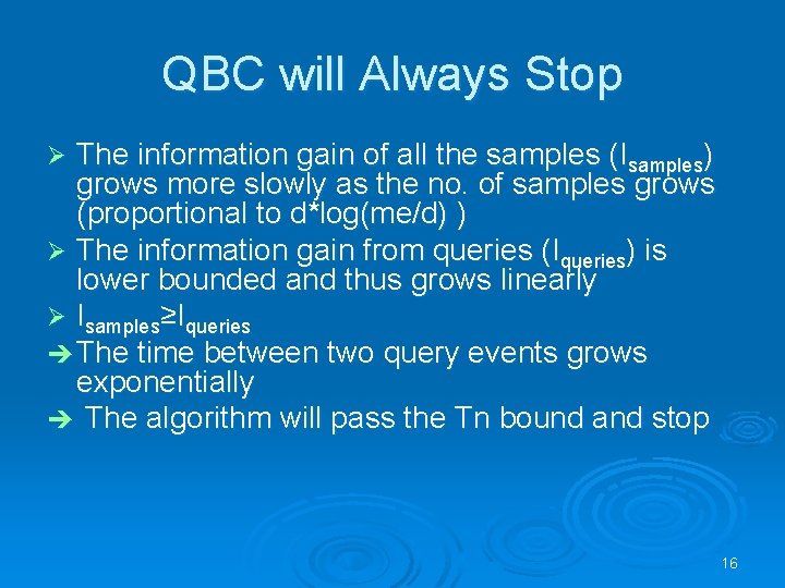
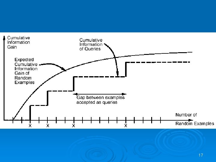
QBC will Always Stop The information gain of all the samples (Isamples) grows more slowly as the no. of samples grows (proportional to d*log(me/d) ) Ø The information gain from queries (Iqueries) is lower bounded and thus grows linearly Ø Isamples≥Iqueries The time between two query events grows exponentially The algorithm will pass the Tn bound and stop Ø 16

17

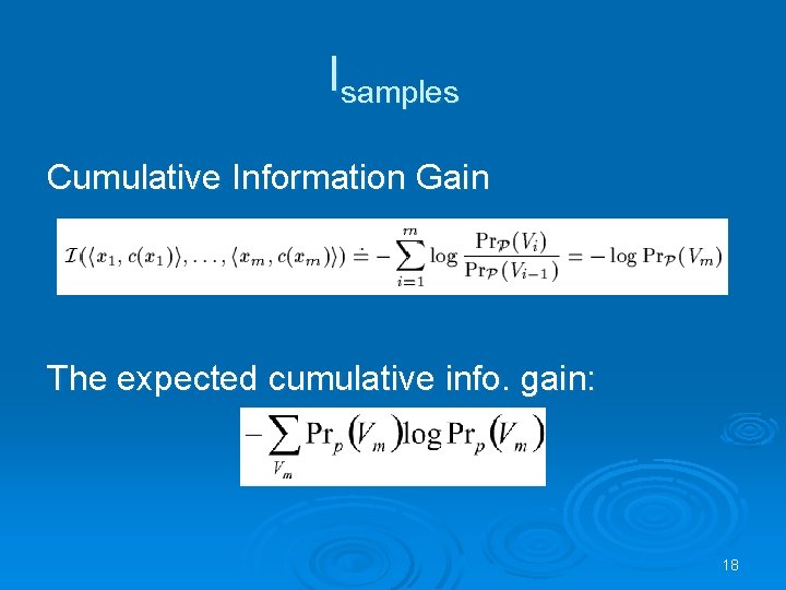
Isamples Cumulative Information Gain The expected cumulative info. gain: 18

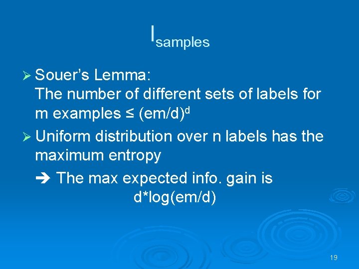
Isamples Ø Souer’s Lemma: The number of different sets of labels for m examples ≤ (em/d)d Ø Uniform distribution over n labels has the maximum entropy The max expected info. gain is d*log(em/d) 19

The Error Probability Ø Definition: Pr(h(x) ≠ c(x)); h, c~PVS Ø This is exactly the probability of querying a sample in QBC This is stopping condition in QBC 20

Before We Go Further… The basic intuition - gaining more information by choosing examples that cut the VS to parts of similar size Ø This condition is not sufficient Ø If there exists a lower bound on the expected info. gain QBC will work Ø The error bound in QBC is based on the analogy between the problem definition and Gibbs, not on the VS cutting. Ø 21

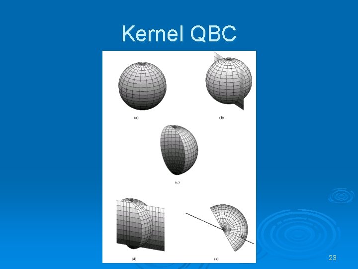
But in Practice… Ø Proved for linear separators if the sample space and VS distributions are uniform. Ø Is the setting realistic? Ø Implementation of Gibbs by Sampling from Convex Bodies 22

Kernel QBC 23

What about Noise? Ø In practice labels might be noisy Ø Active learners are sensitive to noise since they try to minimize redundancy 24

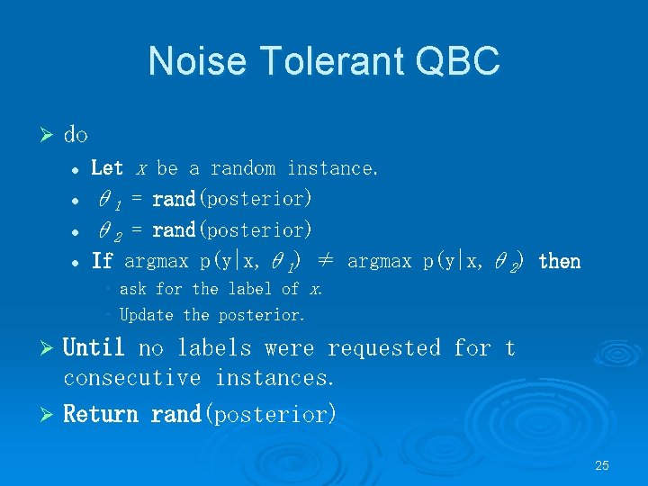
Noise Tolerant QBC Ø do l l Let x be a random instance. θ 1 = rand(posterior) θ 2 = rand(posterior) If argmax p(y|x, θ 1) ≠ argmax p(y|x, θ 2) then • ask for the label of x. • Update the posterior. Until no labels were requested for t consecutive instances. Ø Return rand(posterior) Ø 25

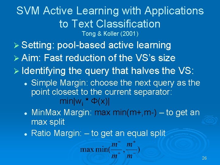
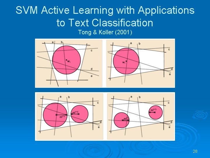
SVM Active Learning with Applications to Text Classification Tong & Koller (2001) Ø Setting: pool-based active learning Ø Aim: Fast reduction of the VS’s size Ø Identifying the query that halves the VS: l l l Simple Margin: choose the next query as the point closest to the current separator: min|wi * Φ(x)| Min. Max Margin: max min(m+, m-) – to get an max split Ratio Margin: – to get an equal split 26

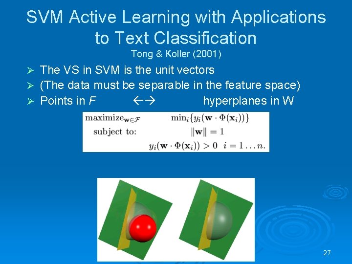
SVM Active Learning with Applications to Text Classification Tong & Koller (2001) The VS in SVM is the unit vectors Ø (The data must be separable in the feature space) Ø Points in F hyperplanes in W Ø 27

SVM Active Learning with Applications to Text Classification Tong & Koller (2001) 28

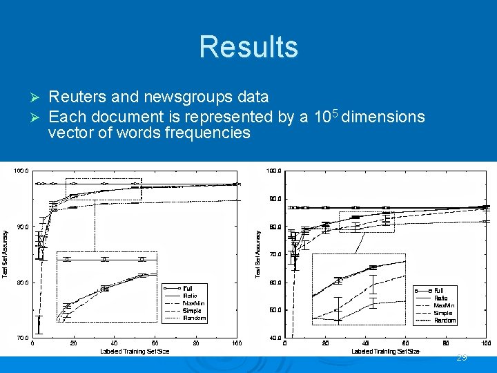
Results Ø Ø Reuters and newsgroups data Each document is represented by a 105 dimensions vector of words frequencies 29

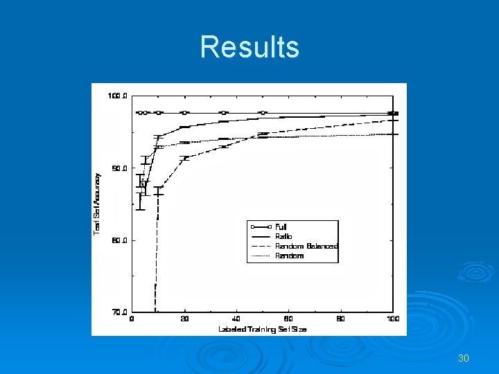
Results 30

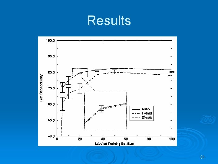
Results 31

What’s next… Ø Theory meet practice Ø New methods (other than cutting the VS)… Ø Generative setting (“committee based sampling for training probabilistic classifiers”, Engelson, 1995) Ø Interesting applications 32

33