ACN Term Project Paper Review ONE MORE BIT

ACN Term Project – Paper Review ONE MORE BIT IS ENOUGH

Introduction From IEEE/ACM Transactions on Networking Because the title is cool! A newly proposed congestion control protocol

High BDP Networks Bandwidth-Delay Product Link capacity times end-to-end delay time e. g. , 100 Mbps x 200 ms = 400 kb = 50 k. B The amount of data “on the air” Transmitted but not yet received Transmitted but not yet ACKed Lack of knowledge about network state
 Drawbacks Low link utilization High packet loss rate Queuing")
TCP Congestion Control Additive-Increase-Multiplicative-Decrease (AIMD) Drawbacks Low link utilization High packet loss rate Queuing delay at bottleneck routers Periodical increase in end-to-end delay

Objectives High link utilization Low persistent bottleneck queue length Almost zero congestion-caused packet loss Fairness among competing flows

Network Feedback Congestion notification is not enough AQM/ECN e. Xplicit Control Protocol, XCP Having routers estimate the fair flow rate �Based on sparse bandwidth, per flow state �Excellent performance Drawbacks �High computational cost �Not compatible with current IP header

XCP “…step back and rethink Internet congestion control without caring about backward compatibility and deployment. ” Proposed the “Congestion header” includes Sender’s current cwnd Sender’s rtt estimate Initialized to sender’s demands, later adjusted by the routers May introduce limits in order to adapt to IP header using multiple bits (e. g. , 8 bits)

Solution Spectrum End-to-end control Network feedback

VCP Variable-structure congestion Control Protocol

Abstract At router Periodically computes a “load factor” and classified in to three regions Encodes in the ECN bits At end-host The receiver echoes the congestion information back to the sender via ACK packets The sender apply different window policy according to the load factor
 High-load: use Additive Increase")
Load Factor Regions Three levels Low-load: use Multiplicative Increase (MI) High-load: use Additive Increase (AI) Overload: use Multiplicative Decrease (MD)

Benefits Exponentially ramp up bandwidth to improve network utilization quickly in low load Provides long-term fairness amongst the competing flows in high load Routers maintain no per-flow state Compatible with current IP header

Simple Demo

Design Guidelines Simple is the best Decouple efficiency control and fairness control They have different levels of relative importance in different load regions Use link load factor as the congestion signal Relative ratio of demand capacity Low computational cost Scale free

Some Formulas MI AI MD Load factor

Load Factor Transition Point Tradeoff between achieving high link utilization and responsiveness to congestion Constraints: The transition point should be sufficiently high Perform an MD from an overload state should force the system enter high-load state A single MI step should lift the system into the high-load state when the utilization is marginally lower than the transition point Chose
")
Load Factor Transition Point (Cont. )

Load Factor Estimation Choosing appropriate time interval, Requirements: Large enough in order to deal with the bursty nature of the Internet flow Short enough to avoid queue buildup Based on statistical report, set

AI/MI Parameter Setting Use as is in TCP MI parameter should be proportional to the spare capacity available in the network

Handling RTT Heterogeneity Parameter scaling For MI For AI MD is not affected by the length of the RTT but should perform only once until new load factor is learned

Summary of Parameter Settings

Performance Evaluation

Single Bottleneck Varying bottleneck capacity
 Varying feedback delay")
Single Bottleneck (Cont. ) Varying feedback delay
 Varying the Number of Long-Lived Flows")
Single Bottleneck (Cont. ) Varying the Number of Long-Lived Flows
 Varying the number of shout-lived traffic")
Single Bottleneck (Cont. ) Varying the number of shout-lived traffic

RTT Fairness 30 FTP flows, sharing a single 150 Mbps bottleneck on reverse path forwarding technique Each flow i's RTT is rtti =40+i*rttdelta performs 11 sets of simulations from 0 to 10 ms. When rttdelta =0 ms, all the flow’s RTTs=40 ms, while rttdelta =10 ms, RTTs are in the range of [40 ms, 330 ms].
")
RTT Fairness (Cont. )
 Result: by Jain’s fairness index XCP shows the best consequence")
RTT Fairness (Cont. ) Result: by Jain’s fairness index XCP shows the best consequence by achieving 1 across the whole set of simulations, with the average 98% bottleneck utilization and the 90 -percetile bottleneck queue length is on average 30% of buffer size. VCP’s bottleneck utilization is slightly less(94%), and only 5% bottleneck buffer size.
 A flow with high RTT is bound to have high")
RTT Fairness (Cont. ) A flow with high RTT is bound to have high values for their MI and AI parameters. We place bounds to restrict the actual value of these parameters to prevent the sudden increase of throughput.

Multiple Bottlenecks Using parking-lot topology, 30 long FTP flows traversing all links in the forward directions, and 30 in the reverse directions. Each individual ink has 5 cross FTP flows in the forward direction.

Multiple Bottlenecks Set all links’ one-way propagation delay to 5 ms. The longest path’s round-trip propagation delay is 80 ms. We vary all the bottleneck links' bandwidth from 500 Kbps to 2 Gbps.

Multiple Bottlenecks The bottleneck links' bandwidth vary from 500 Kbps to 2 Gbps.

Multiple Bottlenecks The bottleneck links' bandwidth vary from 500 Kbps to 2 Gbps.

Multiple Bottlenecks The bottleneck links' bandwidth vary from 500 Kbps to 2 Gbps.

Multiple Bottlenecks For all the cases, VCP performs as good as in the single-bottleneck scenarios. It achieves at least 93% average bottleneck utilization, less than 5%buffer-size average queue length and no packet drops at all the bottlenecks. In comparison to XCP, one key difference is that VCP penalizes flows that traverse more bottlenecks.

Multiple Bottlenecks Now we fix all the bottlenecks’ bandwidth to 150 Mbps. Vary the longest path’s round-trip propagation delay from 1 ms to 1000 ms.

Multiple Bottlenecks

Multiple Bottlenecks

Multiple Bottlenecks

Multiple Bottlenecks Again, XCP and VCP outperform all the others. VCP trades a few percent of bottleneck utilization for lower bottleneck queue length. Both VCP and XCP drop no packet for all the simulation cases.

Dynamics Now we study the short-term dynamical performance of VCP

Dynamics Single bottleneck link with a bandwidth of 45 Mbps where we introduce 5 flows into the system, one after another, with starting times separated by 100 s. We also set the RTT values of the five flows to different values. The reverse path has 5 flows that are always active.

Dynamics

Dynamics

Dynamics

Dynamics VCP reallocates bandwidth to new flows whenever they come in without affecting its high utilization or causing large instantaneous queue. However, VCP takes a much longer time than XCP to converge to the fair allocation.

Sudden Demand Change Consider an initial setting of 50 forward FTP flows with varying RTTs (uniformly chosen in the range [60 ms, 158 ms]) sharing a 200 Mbps bottleneck link. There are 50 FTP flows on the reverse path. At t=80 s, 150 new forward FTP flows become active; then they leave at 160 s.

Sudden Demand Change

Sudden Demand Change

Sudden Demand Change

Sudden Demand Change It shows that VCP is robust against and responsive to sudden, considerable traffic demand changes.

Bandwidth Differentiate VCP can provide differentiated bandwidth to competing flows that are on the same path. 10 Mbps bottlenecks shared by 3 FTP flows, rtt 1=60 ms, rtt 2=80 ms, rtt 3=100 ms, and weight ω1=3, ω2=2, ω3=1.

Bandwidth Differentiate

Bandwidth Differentiate

Achievable Weight Range We have a bottleneck of capacity 100 Mbps shared by 10 FTP flows of heterogeneous RTT ranging from 60 ms to 150 ms. There also 10 reverse FTP flows all with unit weight.
, #5(RTT=100 ms) and #10(RTT=150 ms)")
Bandwidth Differentiate The simulation result of flow #1(RTT=60 ms), #5(RTT=100 ms) and #10(RTT=150 ms) is shown in figure 12(C).

Bandwidth Differentiate

A Fluid Model Now we use the simplified fluid model to analyze the stability, fairness, and convergence properties of VCP. The proof of stability and fairness of VCP is shown in the appendix of the paper.
 RTTs to claim (or")
A Fluid Model Utilization: The VCP protocol takes O(log. C) RTTs to claim (or release) a major part of any spare (or over-used) capacity C.
 RTTs to converge onto")
A Fluid Model Fairness: The VCP protocol takes O(P*log. Pdelta) RTTs to converge onto fairness for any link, where P is the per-flow bandwidth-delay product, and Pdelta is the largest congestion window difference between flows sharing that link (Pdelta >1).

Discussions

Discussions VCP switches between MI, AI and MD modes based on load factor, so there are natural concerns with respects to the impact of these switches on the system stability, efficiency, and fairness, particularly in systems with highly heterogeneous RTTs. We also discuss the TCPfriendliness and incremental deployment issues.

Stability under Heterogeneous Delays In normal circumstances, VCP makes a transition to MD only from AI. Even if VCP switches directly from MD to MI, if the demand traffic at the router does not change significantly, VCP will eventually slide back into AI. We set the load factor transition point and set MD parameter

Influences of Mode Sliding While MI enables VCP to quickly reach high link utilization, VCP needs also to make sure that the system remains in this state. VCP achieves this goal is the scaling of the MI/AI parameters for flows with different RTTs.

Influences of Mode Sliding There are two major concerns with respect to fairness. First, a flow with a small RTT probes the network faster than a flow with a large RTT. Second, it will take longer for a large-RTT flow to switch from MI to AI than a small-RTT flow.

Influences of Mode Sliding The large-RTT flow may have an unfair advantage. VCP addresses the first issue by using the RTT scaling mechanism.

Stability under Heterogeneous Delays

TCP-Friendliness A VCP flow is TCP-friendly if: with a competing TCP flow that in the steady state, the throughput of the TCP flow matches what it would when competing with a normal TCP flow. VCP operates with AIMD in steady state, it is straight-forward to tailor it to exhibit TCPfriendly behavior.

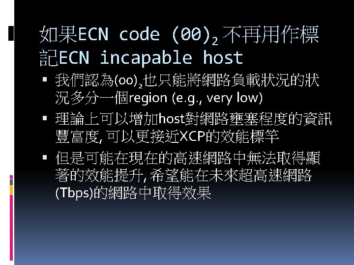
TCP-Friendliness For TCP sources, in order to accordance with the ECN proposal, the encoded load factors (01)2 and (10)2 correspond to no congestion, while (11)2 to congestion.

Incremental Deployment It does not need a new field in the IP header. VCP is made TCP-friendly. The VCP router is scalable in that it does not keep any per-flow state. Its algorithm complexity is very low.

Summary

Summary VCP is a: simple low-complexity high utilization negligible packet loss rate low persistent bottleneck queue reasonable fairness congestion control protocol for high BDP networks.

Future Work it would be interesting to study if we can design a pure end-to-end VCP without any explicit congestion information from network.

Future Work One possibility would be to use packet loss to differentiate between overload and high-load regions and to use RTT variation to differentiate between high-load and low-load regions. While in this paper we evaluate VCP through extensive simulations, ultimately, only a real implementation and deployment will allow us to asses the strengths and limitations of VCP.

Thank You!

IP Header – ECN bits back

Jain’s Fairness Index back

Parking–lot Topology Always find the topologically nearest server to request for service until the server’s queue is full. back
- Slides: 81