Accrued Interest and Quoted Bond Price n n
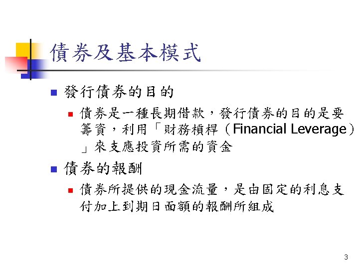
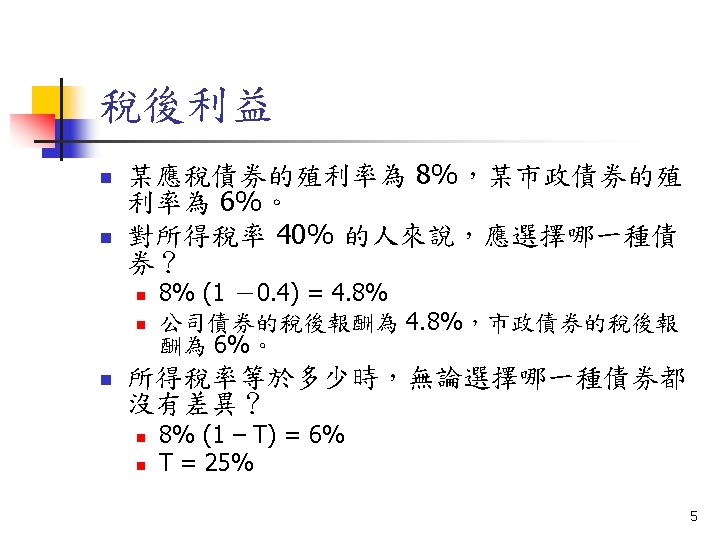

Accrued Interest and Quoted Bond Price n n If a bond is purchased between coupon payments, the buyer must pay the seller for accrued interest. The quoted price does not include the interest that accrues between coupon payment dates. 6

Accrued Interest Example n n For example, if 40 days have passed since the last coupon payment, and there are 182 days in the semiannual coupon period, the seller is entitled to a payment of accrued interest of 40/182 of the semiannual coupon. Supposed that the coupon rate is 8%, the quoted price of the bond is $990, then the invoice price will be $990+$8. 79=$998. 79. 7

Growth of Invested Funds 18

Growth of Invested Funds 19

Default Risk and Yield Example Expected YTM Stated YTM Coupon payment $45 # of semiannual periods 20 periods Final payment $700 $1, 000 Price $750 Yield 11. 6% 13. 7% 20
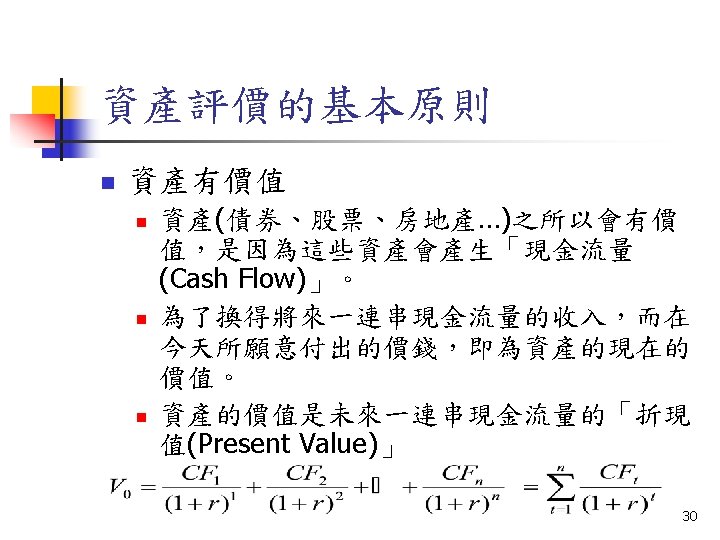

Bond Pricing Bond value = present value of coupons + present value of par value PB = Ct = T = y = Price of the bond interest or coupon payments number of periods to maturity semi-annual discount rate or the semiannual yield to maturity 31
 32")
Bond Pricing (cont. ) 32

The Price of a 30 -Year Zero-Coupon Bond over Time at a Yield to Maturity of 10% 35

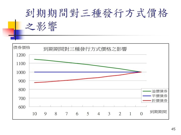
溢價債券價格計算 c=8%, T=10, F=1, 000, r=6% 年 0 票面 利息 溢價債券 1 2 3 4 5 6 7 8 9 10 80 80 80 面值 1000 現金 流量 80 80 80 1080 折現 因子 0. 94 0. 89 0. 84 0. 79 0. 75 0. 70 0. 67 0. 63 0. 59 0. 56 折現 值 75. 5 71. 20 67. 17 63. 37 59. 78 56. 40 53. 20 50. 19 47. 35 603. 07 折現 值和 1147. 202 42

平價債券價格計算 c=8%, T=10, F=1, 000, r=8% 年 0 票面 利息 平價債券 1 2 3 4 5 6 7 8 9 10 80 80 80 面值 1000 現金 流量 80 80 80 1080 折現 因子 0. 93 0. 86 0. 79 0. 74 0. 68 0. 63 0. 58 0. 54 0. 50 0. 46 折現 值 74. 07 68. 59 63. 51 58. 80 54. 45 50. 41 46. 68 43. 22 40. 02 500. 25 折現 值和 1000 43

折價債券價格計算 c=8%, T=10, F=1, 000, r=10% 年 0 票面 利息 折價債券 1 2 3 4 5 6 7 8 9 10 80 80 80 面值 1000 現金 流量 80 80 80 1080 折現 因子 0. 91 0. 83 0. 75 0. 68 0. 62 0. 56 0. 51 0. 47 0. 42 0. 39 60. 11 54. 6 4 49. 67 45. 1 6 41. 05 37. 32 33. 93 416. 39 折現 值和 877. 1087 72. 73 66. 12 44

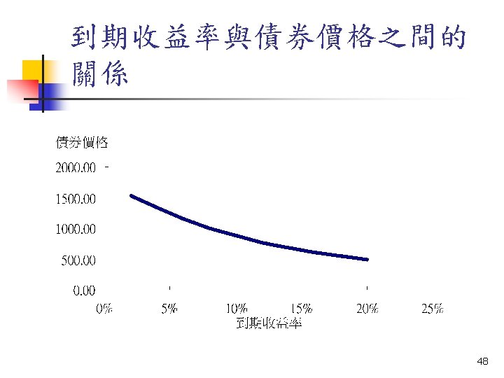
Yield to Maturity Solve the bond formula for y 47
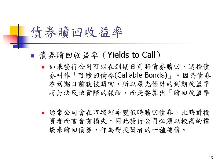

Yield to Call n How should we measure average rate of return for bonds subject to a call provision? n Yield to first call Yield to maturity Coupon payment $40 # of semiannual periods 20 periods 60 periods Final payment $1, 100 $1, 000 Price $1, 150 Yield 6. 64% 6. 82% 50

Bond Prices: Callable and Straight Debt 51

Values of Callable Bonds Compared with Straight Bonds 52
 n")
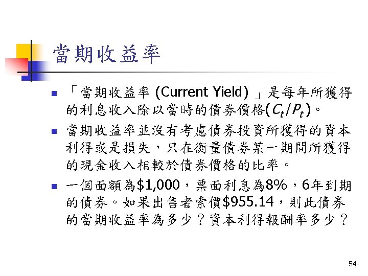
Bond Price over Time n YTM = current yield + capital gain (loss) n Coupon rate < market interest rate n n Discount bond Bond price is lower than face value n n Capital gain Coupon rate > market interest rate n n Premium bond Bond price is higher than face value n Capital loss 55
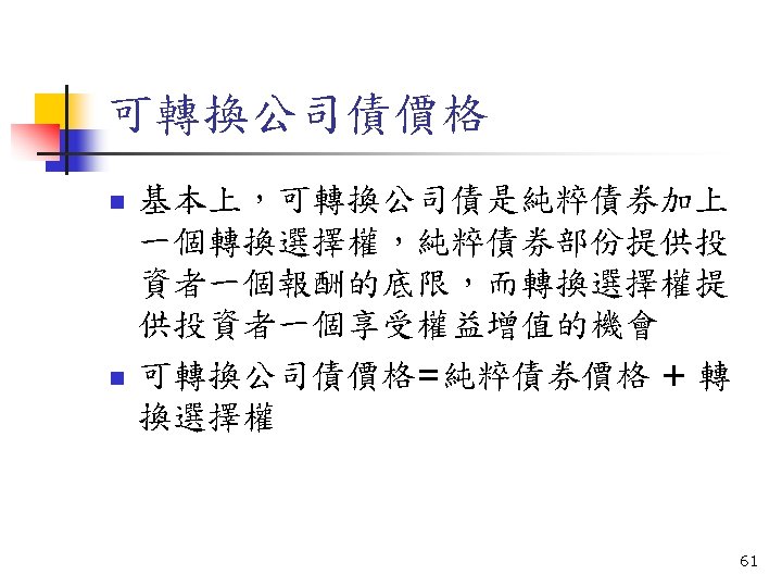

Value of a Convertible Bond as a Function of Stock Price 62

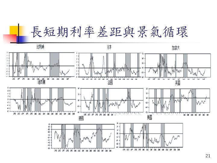
Term Structure n n Should we use the same constant interest rate to discount cash flows of any maturity? Why the longer-term bonds usually offer higher YTM? n n Riskier Investors expect interest rates to rise 64

Term Structure of Interest Rates n n The relationship between yield to maturity and maturity. The yield curve is a graph that displays the relationship between yield and maturity. Information on expected future short term rates can be implied from yield curve. Two major theories are proposed to explain the observed yield curve. 65

Treasury Yield Curves 66

Theories of Term Structure n n Expectations Liquidity Preference n Upward bias over expectations 67

Expectations Theory n n n Observed long-term rate is a function of today’s short-term rate and expected future short-term rates. Forward rates that are calculated from the yield on long-term securities are market consensus expected future short-term rates. Liquidity premiums are zero. 68

Liquidity Preference Theory n Long-term bonds are more risky. n n n Investors will demand a premium for the risk associated with long-term bonds. The yield curve has an upward bias built into the long-term rates because of the risk premium. Forward rates contain a liquidity premium and are not equal to expected future short-term rates. 69

Constant expected short rate 70

Declining expected short rate 71

Declining expected short rate 72

Increasing expected short rate 73
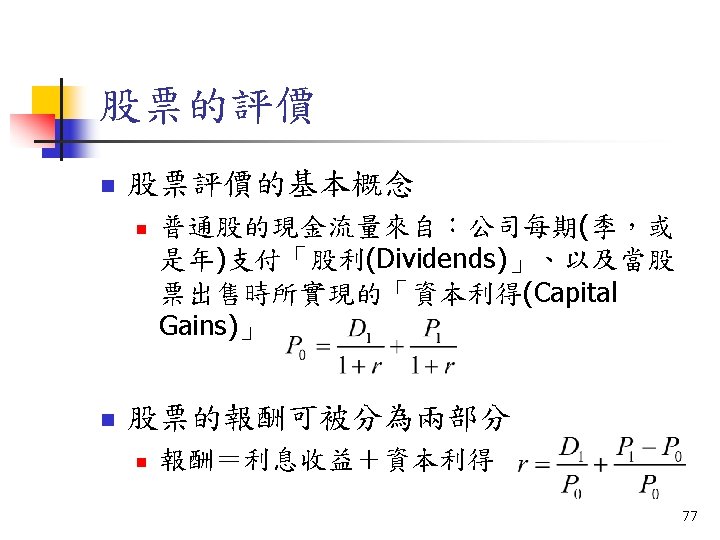
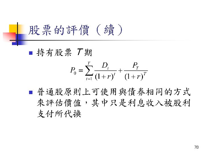

Dividend Discount Models: General Model 79

No Growth DDM n n Stocks that have earnings and dividends that are expected to remain constant. Preferred Stock 80

No Growth DDM Example n n E 1 = D 1 = $5. 00 k = 15% 81

Constant Growth DDM n Dividends are trending upward at a stable growth rate, g 82

Constant Growth DDM Example n n n E 1 = $5. 00 b = 40%, k = 15%, g = 8% d = (1 -b) = 60%, D 1 = $3. 00 83

Table - Financial Ratios in Two Industries 84

Life Cycles and Multistage Growth DDM n Dividends per share grow at several different rates as the firm matures. 85

Life Cycles and Multistage Growth DDM Example n n D 0 = $2. 00, g 1 = 20%, g 2 = 5% T = 3, k = 15% 86

Discounted Cash Flow Formula n For a stock whose market price equals its intrinsic value n n The expected holding period return This formula offers a means to infer the market capitalization rate of a stock 87

Estimating Dividend Growth Rates n n ROE = Return on Equity for the firm b = plowback or retention percentage rate = (1 - dividend payout percentage rate) 88

Present Value of Growth Opportunities n n If the stock price equals its IV, growth rate is sustained, the stock should sell at If all earnings paid out as dividends, price should be lower (assuming growth opportunities exist) 89

Investment opportunities n Cash Cow, Inc. n n Perpetual dividend flow of $5 K = 12. 5% Pc = $5 / 0. 125 = $40 Growth Prospects n n n ROE = 15%, b = 60%, D 1 = 2 g = 0. 15 * 0. 6 = 0. 09 Pg = $2 / (0. 125 -0. 09) = $57. 14 90

Dividend Growth for Two Earnings Reinvestment Policies 91

Growth & No Growth Components of Value n No growth n With growth n PVGO = present value of growth opportunities 92

Partitioning Value Example n ROE = 20%, d = 60%, E 1 = $5. 00, D 1 = $3. 00, k = 15% g = 0. 20 * (1 -0. 60) = 8% n Value with growth n No growth component value n Present value of growth opportunities n 93

Price Earnings Ratios n n The ratio of a stock’s price to its earnings per share. P/E Ratios are a function of two factors n n n Required Rates of Return (k) Expected growth in Dividends Growth opportunities are reflected in P/E ratio 94

P/E Ratio: No Expected Growth n E 1 - expected earnings for next year n n E 1 is equal to D 1 under no growth k - required rate of return 95

Numerical Example: No Growth n E 0 = $2. 50, g = 0, k = 12. 5% 96

P/E Ratio with Constant Growth 97

Numerical Example with Growth n n E 0 = $2. 50, k = 12. 5%, b = 60% ROE = 15%, g=9% E 1 = $2. 73, D 1 = $1. 09 98

Effect of ROE and Plowback on Growth and the P/E Ratio 99

P/E Ratios and Stock Risk n Holding all else equal n n n Riskier stocks will have lower P/E multiples Riskier firms will have higher required rates of return (higher values of k) Higher values of k, therefore, the P/E multiple will be lower 100
 n 承銷方法 n n 包銷制(Firm Commitment Offerings) 代銷制(Best Effort Offerings) 104")
股票上市(續) n 承銷方法 n n 包銷制(Firm Commitment Offerings) 代銷制(Best Effort Offerings) 104
- Slides: 104