Acceleration Structures CS 148 Introduction to Computer Graphics

Acceleration Structures CS 148: Introduction to Computer Graphics and Imaging Image: "BL Object 5" by Douglas Eichenberg (2003)

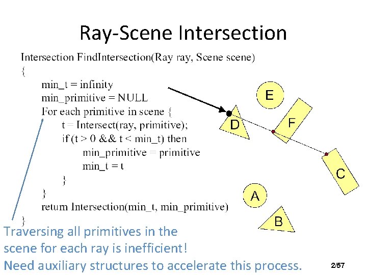
Ray-Scene Intersection Traversing all primitives in the scene for each ray is inefficient! Need auxiliary structures to accelerate this process. 2/57

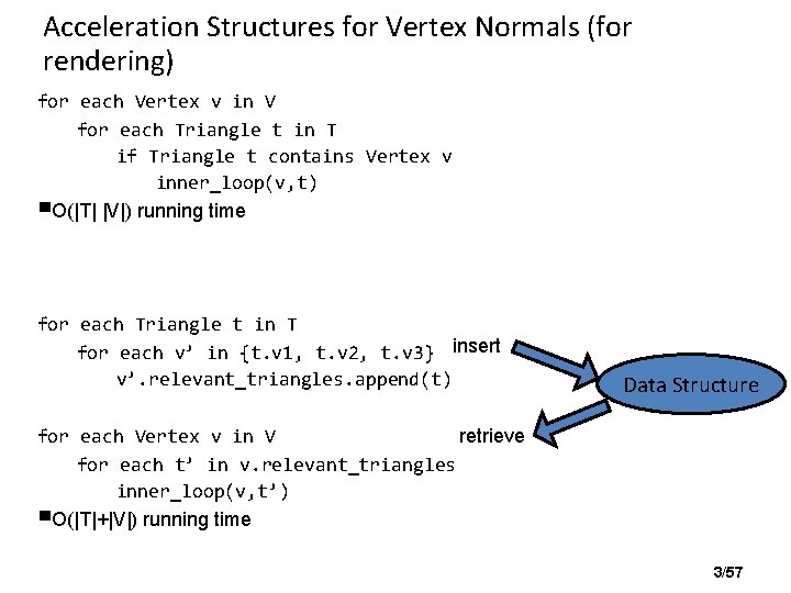
Acceleration Structures for Vertex Normals (for rendering) for each Vertex v in V for each Triangle t in T if Triangle t contains Vertex v inner_loop(v, t) ￭O(|T| |V|) running time for each Triangle t in T for each v’ in {t. v 1, t. v 2, t. v 3} insert v’. relevant_triangles. append(t) Data Structure for each Vertex v in V retrieve for each t’ in v. relevant_triangles inner_loop(v, t’) ￭O(|T|+|V|) running time 3/57

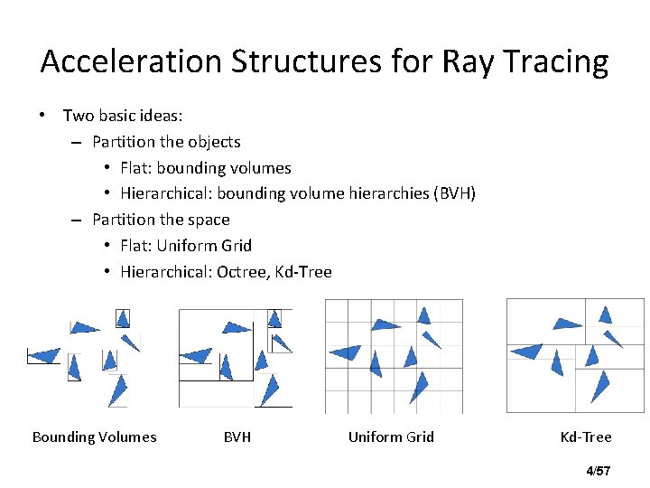
Acceleration Structures for Ray Tracing • Two basic ideas: – Partition the objects • Flat: bounding volumes • Hierarchical: bounding volume hierarchies (BVH) – Partition the space • Flat: Uniform Grid • Hierarchical: Octree, Kd-Tree Bounding Volumes BVH Uniform Grid Kd-Tree 4/57

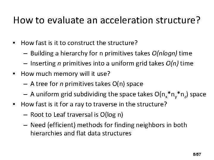
How to evaluate an acceleration structure? • How fast is it to construct the structure? – Building a hierarchy for n primitives takes O(nlogn) time – Inserting n primitives into a uniform grid takes O(n) time • How much memory will it use? – A tree for n primitives takes O(n) space – A uniform grid subdividing the space takes O(nx*ny*nz) space • How fast is it for a ray to traverse in the structure? – Root to Leaf traversal is O(log n) – Need (efficient) methods for finding neighbors in both hierarchies and flat data structures 5/57

Bounding Volume • Enclosing each object with a simpler piece of geometry – Sphere, box (axis-aligned, object-aligned) • If the ray does not hit the bounding volume, it cannot hit the enclosed object – Avoid expensive intersection test with the object 6/57

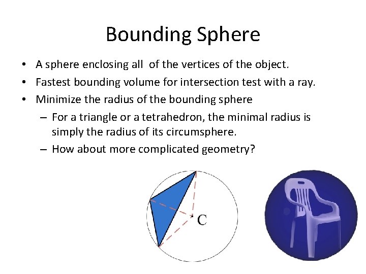
Bounding Sphere • A sphere enclosing all of the vertices of the object. • Fastest bounding volume for intersection test with a ray. • Minimize the radius of the bounding sphere – For a triangle or a tetrahedron, the minimal radius is simply the radius of its circumsphere. – How about more complicated geometry? 7/57

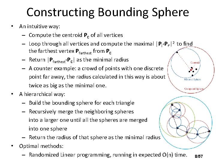
Constructing Bounding Sphere • An intuitive way: – Compute the centroid PC of all vertices – Loop through all vertices and compute the maximal |Pi-PC|2 to find the farthest vertex Pfarthest from PC – Return |Pfarthest-PC| as the minimal radius – A counter example: a crowd of points with one discrete point far away, the radius calculated in this way is about twice as big as the minimal one. • A hierarchical way: – Build the bounding sphere for each triangle – Recursively merge the neighboring spheres into a larger one until all the spheres are merged into one sphere – Return the radius of that sphere as the minimal radius • Optimal methods: – Randomized Linear programming, running in expected O(n) time. 8/57

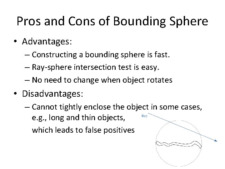
Pros and Cons of Bounding Sphere • Advantages: – Constructing a bounding sphere is fast. – Ray-sphere intersection test is easy. – No need to change when object rotates • Disadvantages: – Cannot tightly enclose the object in some cases, e. g. , long and thin objects, which leads to false positives 9/57

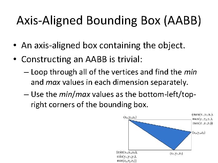
Axis-Aligned Bounding Box (AABB) • An axis-aligned box containing the object. • Constructing an AABB is trivial: – Loop through all of the vertices and find the min and max values in each dimension separately. – Use the min/max values as the bottom-left/topright corners of the bounding box. 10/57

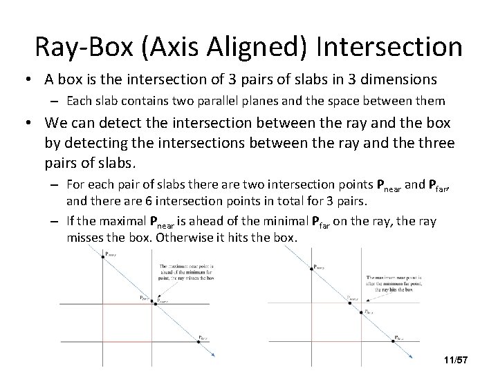
Ray-Box (Axis Aligned) Intersection • A box is the intersection of 3 pairs of slabs in 3 dimensions – Each slab contains two parallel planes and the space between them • We can detect the intersection between the ray and the box by detecting the intersections between the ray and the three pairs of slabs. – For each pair of slabs there are two intersection points Pnear and Pfar, and there are 6 intersection points in total for 3 pairs. – If the maximal Pnear is ahead of the minimal Pfar on the ray, the ray misses the box. Otherwise it hits the box. 11/57

Pseudocode float Ray. Box. Intersection (Ray ray, Box box, Interval [tmin, tmax]) { calculate tnear, x , tfar, x , tnear, y , tfar, y , tnear, z , tfar, z on 3 axes; tnear=max(tnear, x , tnear, y , tnear, z); tfar=min(tfar, x , tfar, y , tfar, z); if(tnear<tfar && tnear>=tmin && tnear<=tmax){ return tnear; ////report intersection at tnear } else{ return -1; ////no intersection } } 12/57

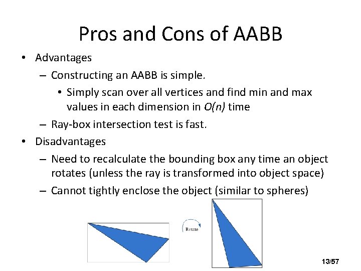
Pros and Cons of AABB • Advantages – Constructing an AABB is simple. • Simply scan over all vertices and find min and max values in each dimension in O(n) time – Ray-box intersection test is fast. • Disadvantages – Need to recalculate the bounding box any time an object rotates (unless the ray is transformed into object space) – Cannot tightly enclose the object (similar to spheres) 13/57

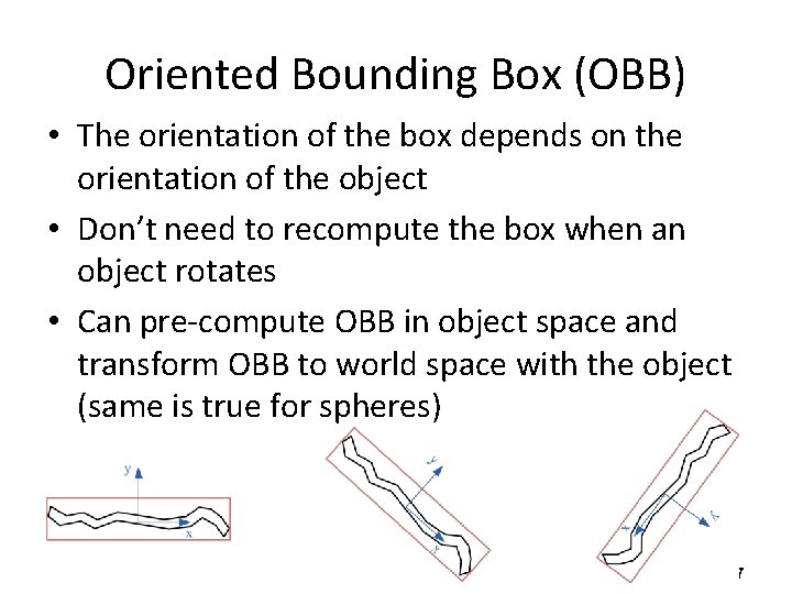
Oriented Bounding Box (OBB) • The orientation of the box depends on the orientation of the object • Don’t need to recompute the box when an object rotates • Can pre-compute OBB in object space and transform OBB to world space with the object (same is true for spheres) 14/57

Constructing OBB • How to compute the orientation of the object? – Singular Value Decomposition – Compute the covariance matrix and the eigenvalues and the corresponding eigenvectors of the 3 x 3 matrix – Using these eigenvectors as the basis of the local coordinate system of the bounding box 15/57

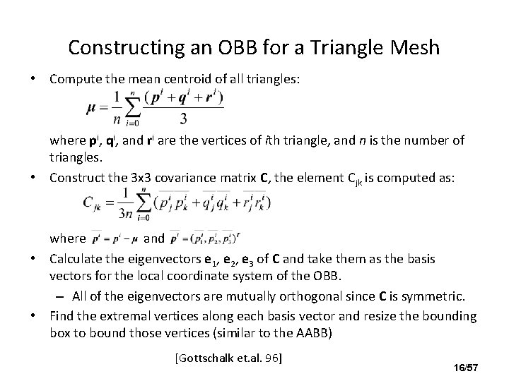
Constructing an OBB for a Triangle Mesh • Compute the mean centroid of all triangles: where pi, qi, and ri are the vertices of ith triangle, and n is the number of triangles. • Construct the 3 x 3 covariance matrix C, the element Cjk is computed as: where and • Calculate the eigenvectors e 1, e 2, e 3 of C and take them as the basis vectors for the local coordinate system of the OBB. – All of the eigenvectors are mutually orthogonal since C is symmetric. • Find the extremal vertices along each basis vector and resize the bounding box to bound those vertices (similar to the AABB) [Gottschalk et. al. 96] 16/57

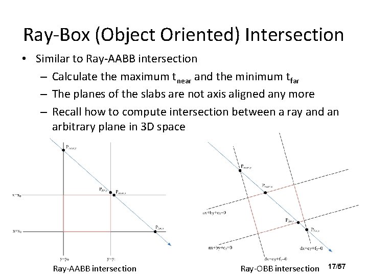
Ray-Box (Object Oriented) Intersection • Similar to Ray-AABB intersection – Calculate the maximum tnear and the minimum tfar – The planes of the slabs are not axis aligned any more – Recall how to compute intersection between a ray and an arbitrary plane in 3 D space Ray-AABB intersection Ray-OBB intersection 17/57

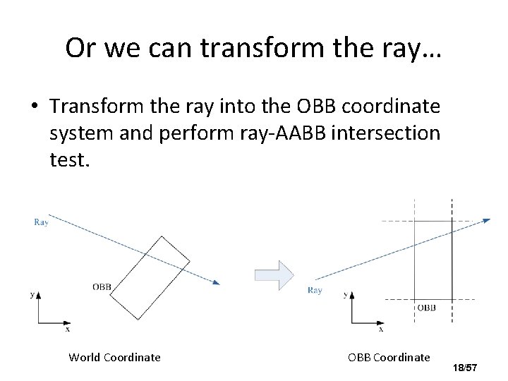
Or we can transform the ray… • Transform the ray into the OBB coordinate system and perform ray-AABB intersection test. World Coordinate OBB Coordinate 18/57

Pros and Cons of OBB • Advantages – Fit the object tighter than AABB • Disadvantages – Extra cost for ray-box intersection – Finding an OBB is computationally expensive (but is done as a precomputation) – Finding the minimal OBB is hard (but an approximation – such as the one we just proposed - is usually good enough) 19/57

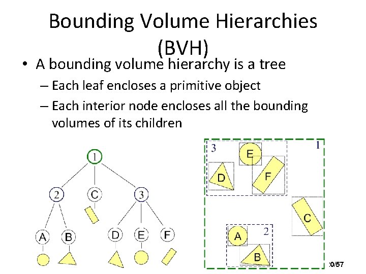
Bounding Volume Hierarchies (BVH) • A bounding volume hierarchy is a tree – Each leaf encloses a primitive object – Each interior node encloses all the bounding volumes of its children 20/57

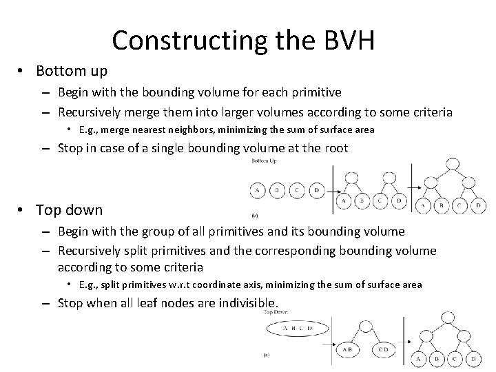
Constructing the BVH • Bottom up – Begin with the bounding volume for each primitive – Recursively merge them into larger volumes according to some criteria • E. g. , merge nearest neighbors, minimizing the sum of surface area – Stop in case of a single bounding volume at the root • Top down – Begin with the group of all primitives and its bounding volume – Recursively split primitives and the corresponding bounding volume according to some criteria • E. g. , split primitives w. r. t coordinate axis, minimizing the sum of surface area – Stop when all leaf nodes are indivisible. 21/57

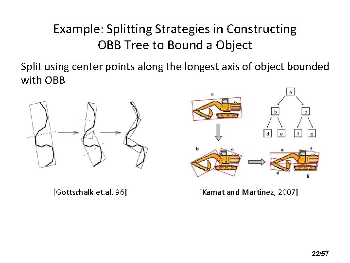
Example: Splitting Strategies in Constructing OBB Tree to Bound a Object Split using center points along the longest axis of object bounded with OBB [Gottschalk et. al. 96] [Kamat and Martinez, 2007] 22/57

Where/When to create the BVHs? • Create the BVH individually for each object – The BVH is in object space – Can be translated with the object and does not need to be updated • Create BVH for unioning together all BVs of all objects in a scene – This global BVH is in the world space – Must be updated whenever something moves in the scene • Do both! 23/57

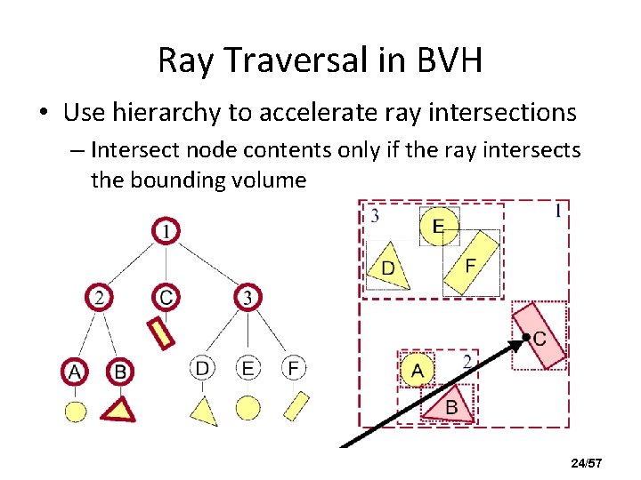
Ray Traversal in BVH • Use hierarchy to accelerate ray intersections – Intersect node contents only if the ray intersects the bounding volume 24/57

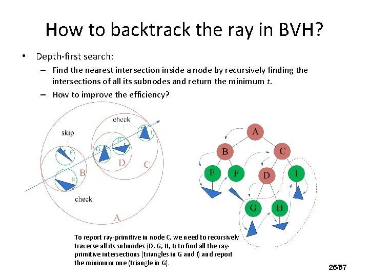
How to backtrack the ray in BVH? • Depth-first search: – Find the nearest intersection inside a node by recursively finding the intersections of all its subnodes and return the minimum t. – How to improve the efficiency? To report ray-primitive in node C, we need to recursively traverse all its subnodes (D, G, H, I) to find all the rayprimitive intersections (triangles in G and I) and report the minimum one (triangle in G). 25/57

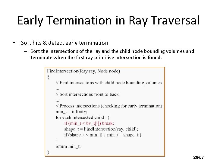
Early Termination in Ray Traversal • Sort hits & detect early termination – Sort the intersections of the ray and the child node bounding volumes and terminate when the first ray-primitive intersection is found. 26/57

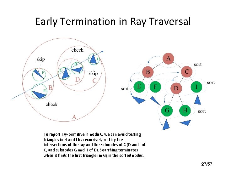
Early Termination in Ray Traversal To report ray-primitive in node C, we can avoid testing triangles in H and I by recursively sorting the intersections of the ray and the subnodes of C (D and I of C, and subnodes G and H of D). Searching terminates when it finds the first triangle (in G) in the sorted nodes. 27/57

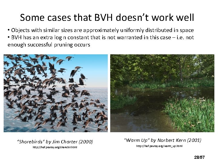
Some cases that BVH doesn’t work well • Objects with similar sizes are approximately uniformly distributed in space • BVH has an extra log n constant that is not warranted in this case – i. e. not enough successful pruning occurs “Shorebirds” by Jim Charter (2000) http: //hof. povray. org/shorebir. html "Warm Up" by Norbert Kern (2001) http: //hof. povray. org/warm_up. html 28/57

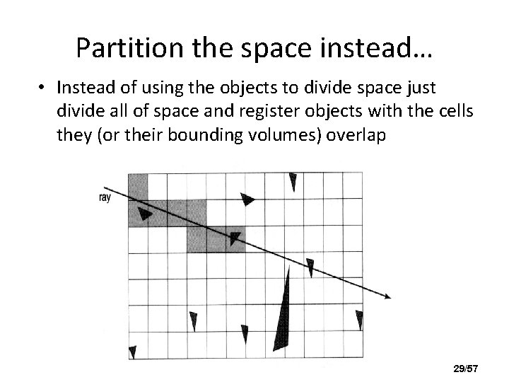
Partition the space instead… • Instead of using the objects to divide space just divide all of space and register objects with the cells they (or their bounding volumes) overlap 29/57

Uniform Grids • Divide 3 D space into nx*ny*nz axis-aligned grid cells • Perform Ray-object intersection test only when the ray hits the grid cell containing the object • The size of the grid cell is crucial to the performance – No speedup if the cell size is too big, no pruning, everything in one cell – A lot of empty cells if the cell size is too small – A practical way to choose cell size is to average the edge lengths of the bounding boxes of all primitives 30/57

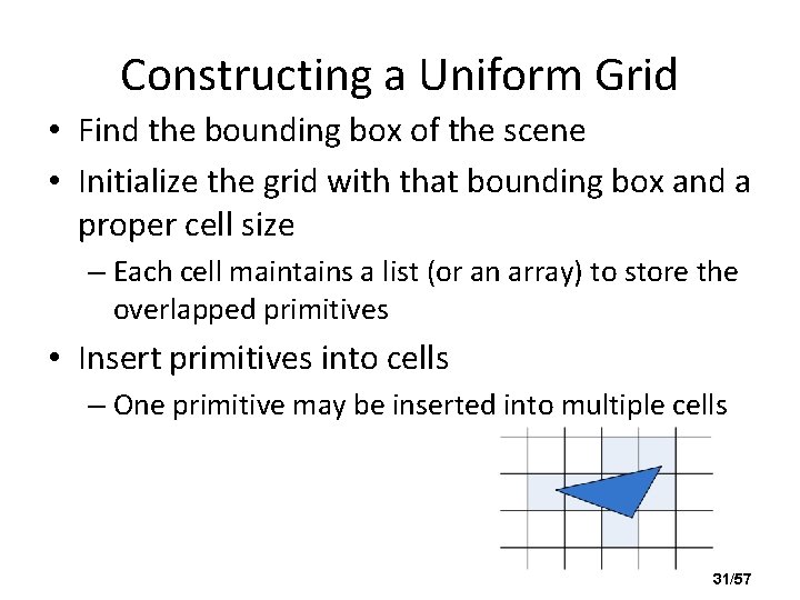
Constructing a Uniform Grid • Find the bounding box of the scene • Initialize the grid with that bounding box and a proper cell size – Each cell maintains a list (or an array) to store the overlapped primitives • Insert primitives into cells – One primitive may be inserted into multiple cells 31/57

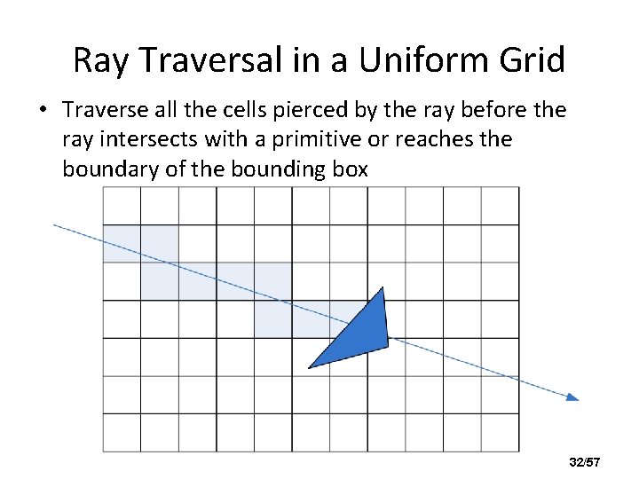
Ray Traversal in a Uniform Grid • Traverse all the cells pierced by the ray before the ray intersects with a primitive or reaches the boundary of the bounding box 32/57

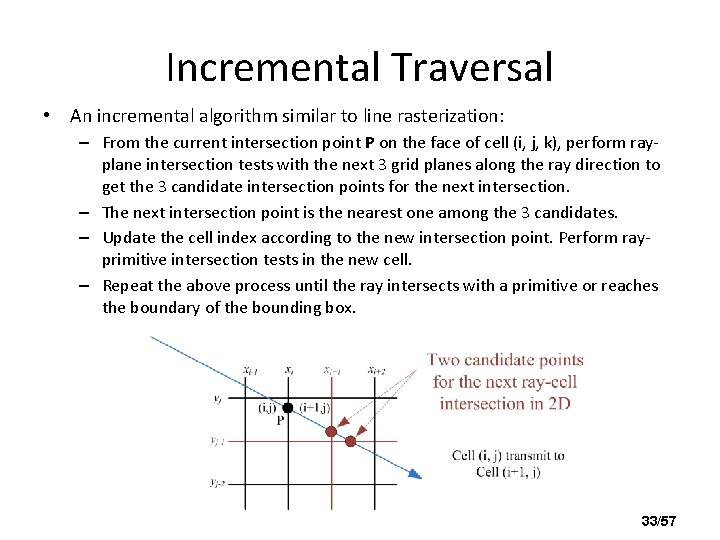
Incremental Traversal • An incremental algorithm similar to line rasterization: – From the current intersection point P on the face of cell (i, j, k), perform rayplane intersection tests with the next 3 grid planes along the ray direction to get the 3 candidate intersection points for the next intersection. – The next intersection point is the nearest one among the 3 candidates. – Update the cell index according to the new intersection point. Perform rayprimitive intersection tests in the new cell. – Repeat the above process until the ray intersects with a primitive or reaches the boundary of the bounding box. 33/57

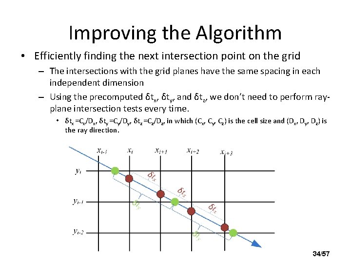
Improving the Algorithm • Efficiently finding the next intersection point on the grid – The intersections with the grid planes have the same spacing in each independent dimension – Using the precomputed δtx, δty, and δtz, we don’t need to perform rayplane intersection tests every time. • δtx =Cx/Dx, δty =Cy/Dy, δtz =Cz/Dz, in which (Cx, Cy, Cz) is the cell size and (Dx, Dy, Dz) is the ray direction. 34/57

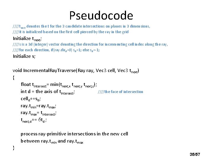
Pseudocode ////tnext denotes the t for the 3 candidate intersections on planes in 3 dimensions, ////it is initialized based on the first cell pierced by the ray in the grid Initialize tnext; ////s is a 3 d (integer) vector denoting the direction for incrementing cell index along the ray, ////for each direction, if(ray. dird>0) sd=1; else sd=-1; Initialize s; void Incremental. Ray. Traverse(Ray ray, Vec 3 cell, Vec 3 tnext) { float tintersect= min(tnext, x tnext, y tnext, z); int d = the axis of tintersect; ////the face of intersection celld+=sd; ray. tmin=ray. tmax; ray. tmax= tintersect; tnext, d+= δtd ; } process ray-primitive intersections in the new cell between ray. tmin and ray. tmax 35/57

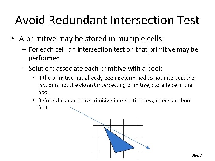
Avoid Redundant Intersection Test • A primitive may be stored in multiple cells: – For each cell, an intersection test on that primitive may be performed – Solution: associate each primitive with a bool: • If the primitive has already been determined to not intersect the ray, or is not the closest intersecting primitive, store false in the bool • Before the actual ray-primitive intersection test, check the bool first 36/57

Pros and Cons of the Uniform Grids • Advantages: – Construction is fast. – Regular Layout, Cache coherent – Ray traversal is easy. • Disadvantages: – Empty cells in a sparse scene will waste memory – Hard to choose the cell size – No adaptivity 37/57

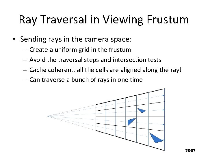
Ray Traversal in Viewing Frustum • Sending rays in the camera space: – – Create a uniform grid in the frustum Avoid the traversal steps and intersection tests Cache coherent, all the cells are aligned along the ray! Can traverse a bunch of rays in one time 38/57

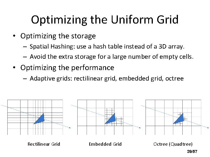
Optimizing the Uniform Grid • Optimizing the storage – Spatial Hashing: use a hash table instead of a 3 D array. – Avoid the extra storage for a large number of empty cells. • Optimizing the performance – Adaptive grids: rectilinear grid, embedded grid, octree Rectilinear Grid Embedded Grid Octree (Quadtree) 39/57

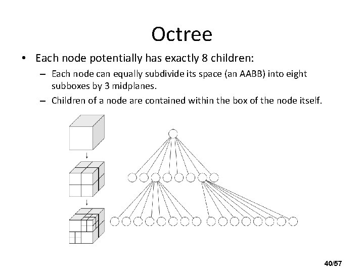
Octree • Each node potentially has exactly 8 children: – Each node can equally subdivide its space (an AABB) into eight subboxes by 3 midplanes. – Children of a node are contained within the box of the node itself. 40/57

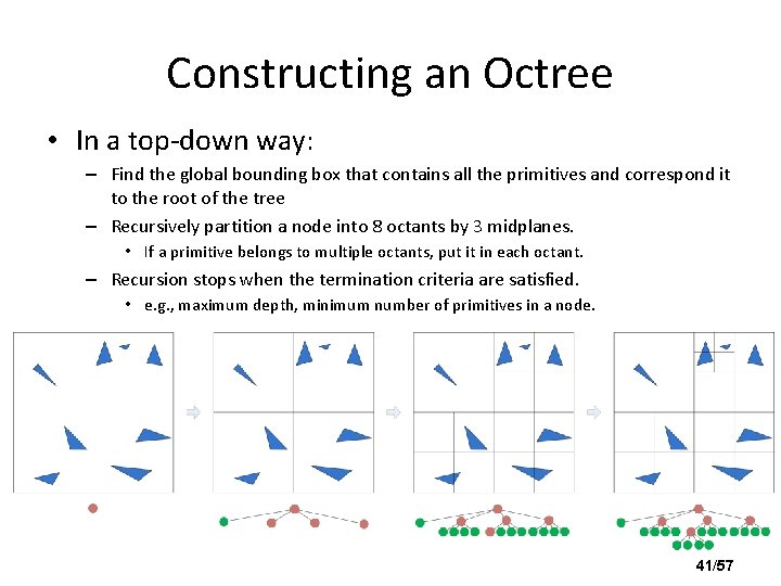
Constructing an Octree • In a top-down way: – Find the global bounding box that contains all the primitives and correspond it to the root of the tree – Recursively partition a node into 8 octants by 3 midplanes. • If a primitive belongs to multiple octants, put it in each octant. – Recursion stops when the termination criteria are satisfied. • e. g. , maximum depth, minimum number of primitives in a node. 41/57

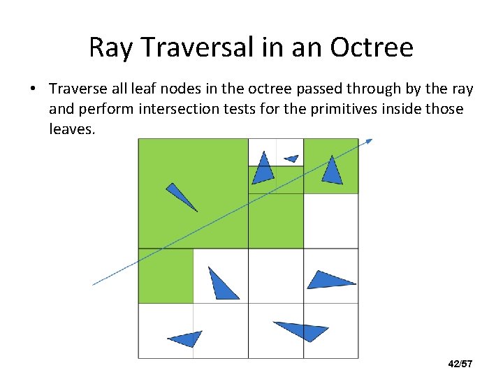
Ray Traversal in an Octree • Traverse all leaf nodes in the octree passed through by the ray and perform intersection tests for the primitives inside those leaves. 42/57

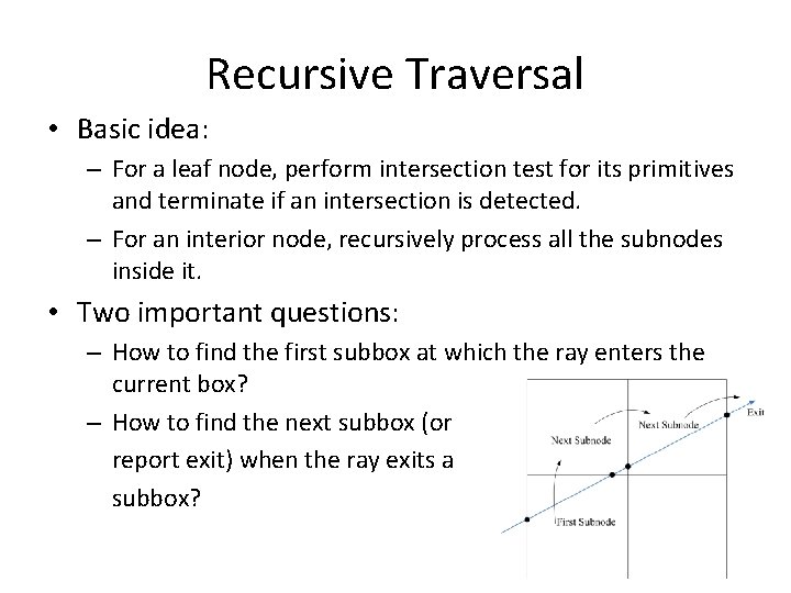
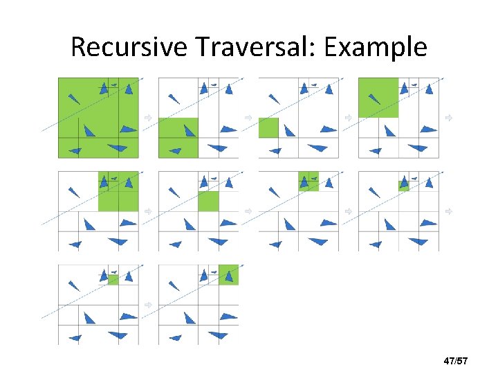
Recursive Traversal • Basic idea: – For a leaf node, perform intersection test for its primitives and terminate if an intersection is detected. – For an interior node, recursively process all the subnodes inside it. • Two important questions: – How to find the first subbox at which the ray enters the current box? – How to find the next subbox (or report exit) when the ray exits a subbox? 43/57

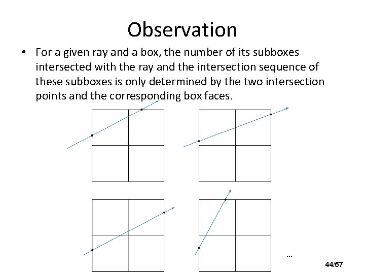
Observation • For a given ray and a box, the number of its subboxes intersected with the ray and the intersection sequence of these subboxes is only determined by the two intersection points and the corresponding box faces. … 44/57

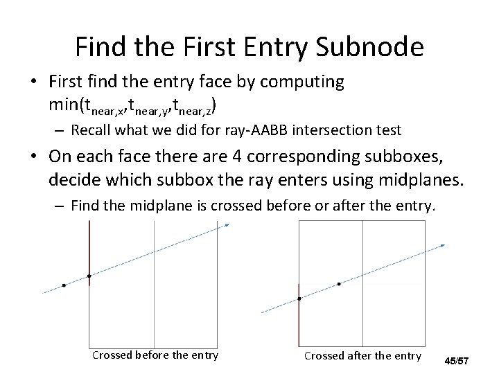
Find the First Entry Subnode • First find the entry face by computing min(tnear, x, tnear, y, tnear, z) – Recall what we did for ray-AABB intersection test • On each face there are 4 corresponding subboxes, decide which subbox the ray enters using midplanes. – Find the midplane is crossed before or after the entry. Crossed before the entry Crossed after the entry 45/57

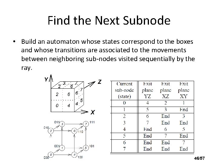
Find the Next Subnode • Build an automaton whose states correspond to the boxes and whose transitions are associated to the movements between neighboring sub-nodes visited sequentially by the ray. 46/57

Recursive Traversal: Example 47/57

Pros and Cons of the Octree • Advantages – Adaptivity – Memory efficiency • Disadvantages – Ray traversal is complicated – Partition strategy is not flexible – Not cache coherent 48/57

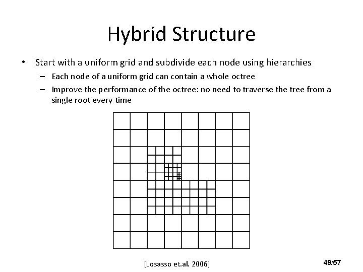
Hybrid Structure • Start with a uniform grid and subdivide each node using hierarchies – Each node of a uniform grid can contain a whole octree – Improve the performance of the octree: no need to traverse the tree from a single root every time [Losasso et. al. 2006] 49/57

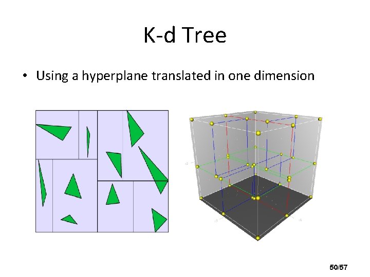
K-d Tree • Using a hyperplane translated in one dimension 50/57

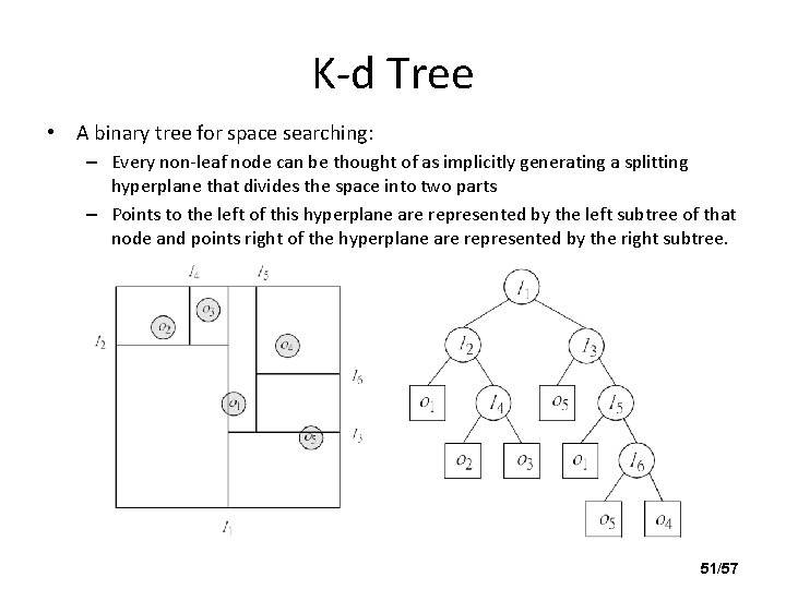
K-d Tree • A binary tree for space searching: – Every non-leaf node can be thought of as implicitly generating a splitting hyperplane that divides the space into two parts – Points to the left of this hyperplane are represented by the left subtree of that node and points right of the hyperplane are represented by the right subtree. 51/57

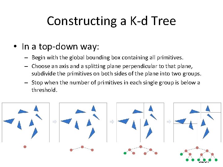
Constructing a K-d Tree • In a top-down way: – Begin with the global bounding box containing all primitives. – Choose an axis and a splitting plane perpendicular to that plane, subdivide the primitives on both sides of the plane into two groups. – Stop when the number of primitives in each single group is below a threshold. 52/57

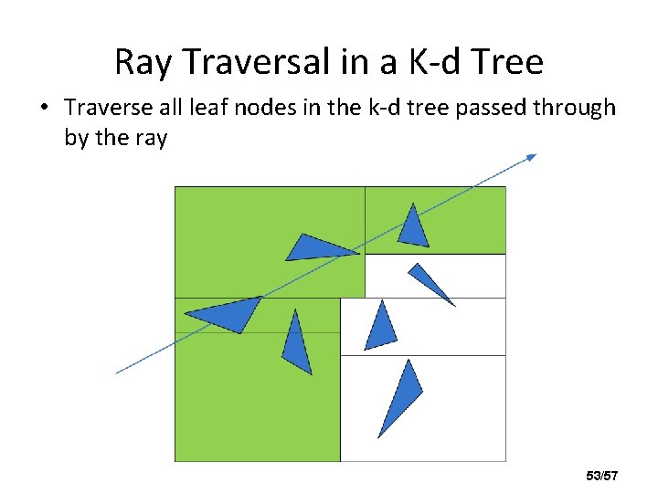
Ray Traversal in a K-d Tree • Traverse all leaf nodes in the k-d tree passed through by the ray 53/57

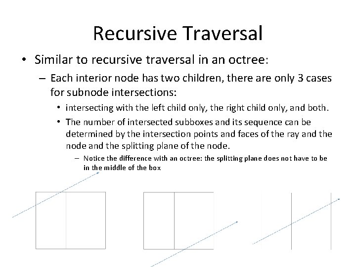
Recursive Traversal • Similar to recursive traversal in an octree: – Each interior node has two children, there are only 3 cases for subnode intersections: • intersecting with the left child only, the right child only, and both. • The number of intersected subboxes and its sequence can be determined by the intersection points and faces of the ray and the node and the splitting plane of the node. – Notice the difference with an octree: the splitting plane does not have to be in the middle of the box 54/57

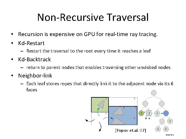
Non-Recursive Traversal • Recursion is expensive on GPU for real-time ray tracing. • Kd-Restart – Restart the traversal to the root every time it reaches a leaf • Kd-Backtrack – return to parent nodes that enables traversing other unvisited nodes • Neighbor-link – Each leaf stores ropes that directly link it to the adjacent node via its 6 faces [Popov et. al. 07] 55/57

Pros and Cons of the K-d Tree • Advantages – Adaptivity – Fast ray traversal • Disadvantages – Construction is complicated 56/57

Partitioning Objects or Space? • Any of the acceleration structures can be applied in both object space and world space in the same manner – When a structure is in the world space, it has to be updated whenever some object or primitive in the structure is transformed – When a structure is in the object space, it can be transformed with the object and does not need to be updated – E. g. , a uniform grid in world space for a bunch of birds with a BVH in object space for each bird 57/57