Abundance of Puget Sound Steelhead near the turn

Abundance of Puget Sound Steelhead near the turn of the 20 th century estimated from commercial catch data Nick Gayeski Wild Fish Conservancy March 14, 2012

Historical abundance of Puget Sound steelhead, Oncorhynchus mykiss, estimated from catch record data • Authors: Nick Gayeski, Bill Mc. Millan, Pat Trotter • Canadian Journal of Fisheries and Aquatic Sciences, vol. 68, pp. 498 -510, March 2011

Project Objectives • Estimate abundance of Puget Sound steelhead based upon: • Commercial catch data for the year of peak catch – 1895 • Historical data regarding regional development to estimate unreported steelhead catch

• Provide a robust historical baseline of PS steelhead abundance to serve as a reference for recovery so as to avoid the ‘shifting baseline syndrome’ • Illustrate how quantitative data can be integrated with qualitative (historical) data to estimate historical abundance while fully accounting for the uncertainty of such estimates

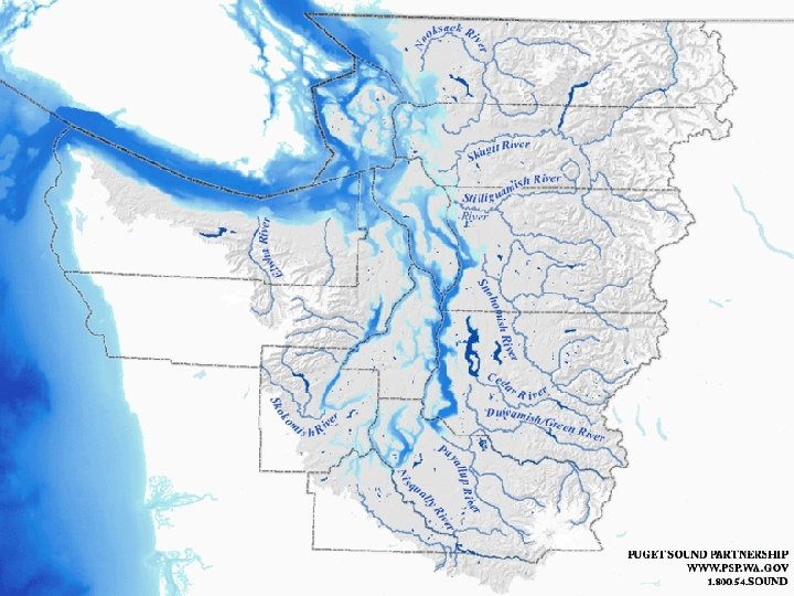
Commercial Catch Data: Available for Five Populations • • • Nooksack Skagit Stillaguamish Snohomish The remaining rivers and streams in Puget Sound

1895 Commercial Catch Data (lbs) • • • Nooksack Skagit Stillaguamish Snohomish Remaining PS TOTAL 660, 160 lbs. 205, 190 lbs. 180, 000 lbs. 401, 620 lbs. 518, 582 lbs. 1, 965, 552 lbs.

Methods 1. Start with reported commercial catch in lbs. 2. Estimate the weight of steelhead in the catch 3. Estimate the unreported catch (tribal, sport, settlers/agricultural) as a proportion of the reported catch From 1 - 3 , estimate the total numerical catch Estimate the total harvest rate on the 1895 run represented by the estimated total catch Do this in a way that accounts for all uncertainties in the estimation procedure

Bayesian Analysis • The uncertainties are accounted for by employing a Bayesian analysis • First, we obtain a distribution of the estimated total numerical catch, T: • T = C*(1+U)/W (eq. 1), where • C = commercial catch in lbs. • U = unreported catch (% of reported) • W = average weight of steelhead (lbs. )

Steelhead weight and unreported catch as a proportion of reported catch • Weight 7 - 9. 5 pounds • • • 0. 10 – 0. 30 0. 50 – 1. 00 Nooksack Skagit Stillaguamish Snohomish Remaining PS

Estimation of the Numerical Catch • • • Randomly draw a large number of values of U and W (10 million) and Apply equation (1) to each. Cumulated values in bins of fixed width to build a histogram of T.

Distribution of Total Catch (Snohomish)

Estimation of the Terminal Run • • • Place a distribution on harvest rate, R, and on total run size, N and calculate P(T|N, R) =(N!/(T!*(N-T)!) *TR*(N-T)(1 -R) (eq. 2) Equation 2 is calculated for 10 million random values of R and N, and the values of T.

Harvest Rate Priors • • • Nooksack: uniform(0. 6, 0. 9) Skagit: uniform(0. 3, 0. 6) Stillaguamish: uniform(0. 4, 0. 7) Snohomish: uniform(0. 4, 0. 7) Remaining: uniform(0. 4, 0. 7)

Terminal Run Size Priors • • • Nooksack: uniform(80000, 225000) Skagit: uniform(50000, 200000) Stillaguamish: uniform(40000, 130000) Snohomish: uniform(90000, 290000) Remaining: uniform(100000, 370000)

Snohomish Prior and Posterior Distributions of Run Size

Snohomish Posterior and Prior Distributions of Harvest Rate

RESULTS

Total Catch Estimates • Population Mean Mode • • • SD Nooksack 96800 91300 9700 Skagit 43900 43300 5300 Stilly. 38500 37700 4700 Snohomish 85900 83700 10400 Remaining 110800 109000 13500 • TOTAL 375900 365000 Cntrl. 90 th%-ile 81700 -- 1135000 -- 53100 31100 – 46600 69500 -- 104300 89400 – 134500 43600 306700 – 452000

Total Run Size Estimates • Population Mean Mode • • • Nooksack Skagit Stilly. Snohomish Remaining • TOTAL SD Cntrl. 90 th%-ile 132600 105600 73700 164500 212100 127800 20400 101400 – 169000 86700 24700 70000 -- 149000 69200 14900 51700 – 100000 153000 33400 114000 -- 224000 185000 43100 148000 – 287700 688500 621700 136500 485100 – 929700

Harvest Rate Estimates • Population Mean • • • Mode SD Cntrl. 90 th%-ile Nooksack Skagit Stilly. Snohomish Remaining 0. 74 0. 43 0. 54 0. 60 0. 31 0. 42 0. 40 0. 09 0. 61 – 0. 31 -0. 41 – 0. 88 0. 58 0. 68 • Grand Mn. • Mn (Totals) 0. 56 0. 55 0. 40 0. 59 0. 09 NA 0. 43 – 0. 36 – 0. 70 0. 63

Comparison to Current Conditions • Two methods of comparison • Compare estimated turn-of-century abundance to NOAA status review estimates for 1980 - 2004 and for 2000 – 2004 • Compare estimates scaled to estimates of lengths of stream accessible to adult winter-run steelhead (fish-per-kilometer)

Current Conditions Population N, 19802004 N, 2000 -04 S FKM, All Years FKM, 5 years Nooksack* 1600 612 2. 6 Skagit 6993. 9 5418. 8 982 7. 12 5. 52 Snohomish 5283 3230. 1 926 5. 71 3. 49 Stillaguamish 1027. 7 550. 2 445 2. 31 1. 24 Rest of PS 6673. 8 4742. 5 4014 1. 69 1. 18 All of PS 21678 15542 6979 3. 1 2. 2

Historical Estimates Population Posterior Mode N Posterior 5 th %ile N SK FKM. Mode N FKM, 5%ile N Nooksack 127800 101400 918 139 110 Skagit 86700 70000 1473 59 48 Snohomish 153000 114000 1389 110 82 Stillaguamis h 69200 51700 667. 5 104 77 Rest of PS 185000 148000 6021 31 25 All of PS 621700 485100 10469 59. 4 46. 3

FKM for Recent Average and Estimated Historical Abundance

Fish-Per-Accessible Stream Km for Historic PS and Situk 1952

CONCLUSIONS • Current abundance is 1% to 4% of the estimated turn-of-century abundance • Habitat currently accessible to adult winterrun steelhead is no less than 67% of what was available at the turn of the century • It is unlikely that habitat loss can explain the majority of this historic decline. • This may indicate that significant recovery is still in the cards!

• Severe impairment of both ecosystem and autecological function • Steelhead have lost significant life history and genetic diversity • Interactions with hatchery fish and loss of salmon abundance in addition to habitat loss and simplification are plausible culprits

Thank You for Your Attention!