A workshop introducing doubly robust estimation of treatment

A workshop introducing doubly robust estimation of treatment effects Michele Jonsson Funk, Ph. D UNC/GSK Center for Excellence in Pharmacoepidemiology University of North Carolina at Chapel Hill

Conflict of Interest Statement n n n Macro development funded by the Agency for Healthcare Research and Quality via a supplemental award to the UNC CERTs (U 18 HS 10397 -07 S 1) Additional support from the UNC/GSK Center for Excellence in Pharmacoepidemiology and Public Health. No potential conflicts of interest with respect to this work. 2

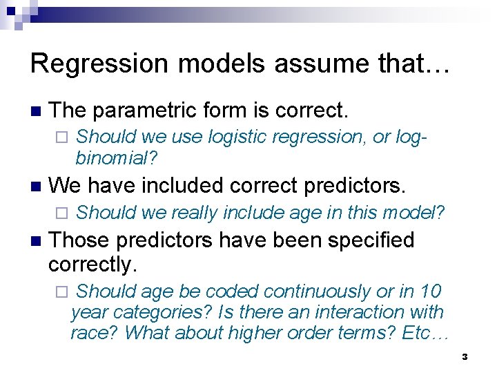
Regression models assume that… n The parametric form is correct. ¨ n We have included correct predictors. ¨ n Should we use logistic regression, or logbinomial? Should we really include age in this model? Those predictors have been specified correctly. ¨ Should age be coded continuously or in 10 year categories? Is there an interaction with race? What about higher order terms? Etc… 3

What if the model is wrong? Lunceford & Davidian, Stat Med, 2004 n Omit a true confounder (extreme example) n True relationships known (simulated data) n Vary associations between n ¨ Risk factor – outcome ¨ Confounder – exposure 4

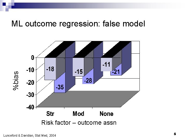
%bias ML outcome regression: false model Risk factor – outcome assn Lunceford & Davidian, Stat Med, 2004 5

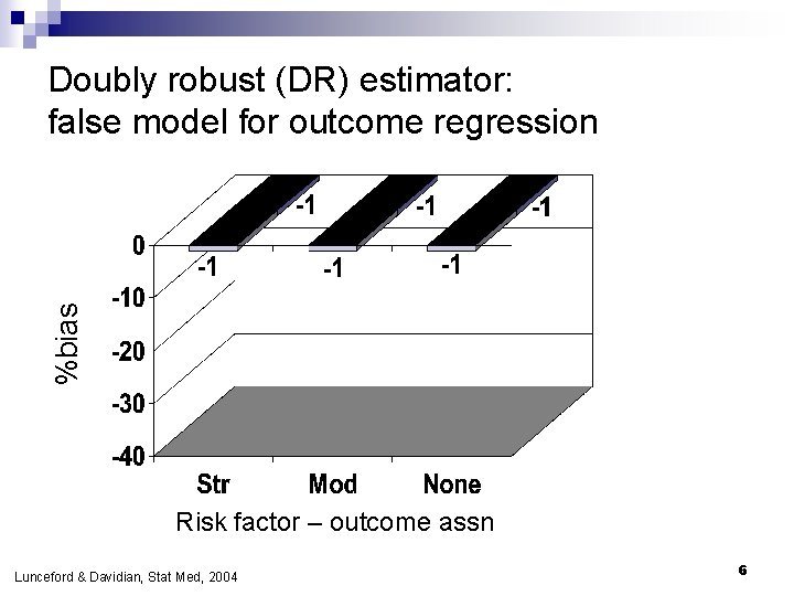
%bias Doubly robust (DR) estimator: false model for outcome regression Risk factor – outcome assn Lunceford & Davidian, Stat Med, 2004 6

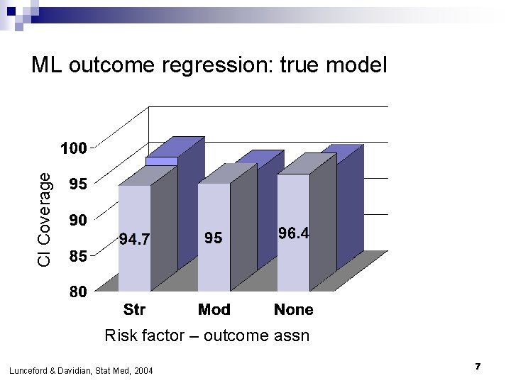
CI Coverage ML outcome regression: true model Risk factor – outcome assn Lunceford & Davidian, Stat Med, 2004 7

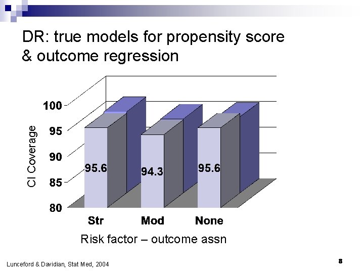
CI Coverage DR: true models for propensity score & outcome regression Risk factor – outcome assn Lunceford & Davidian, Stat Med, 2004 8

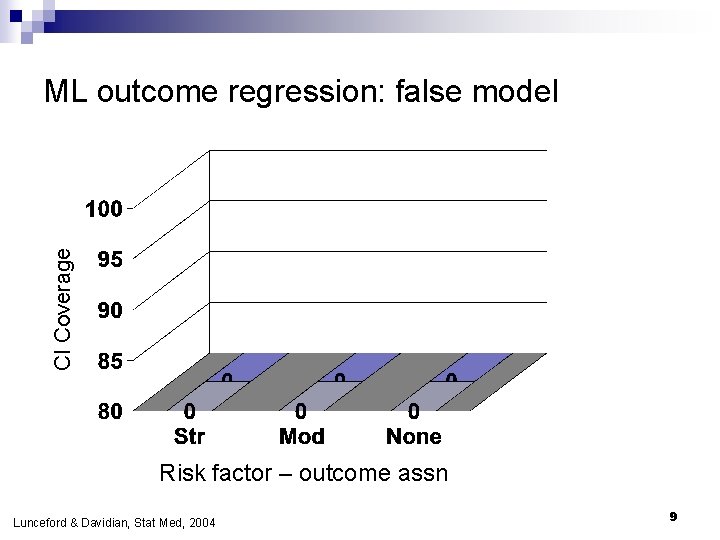
CI Coverage ML outcome regression: false model Risk factor – outcome assn Lunceford & Davidian, Stat Med, 2004 9

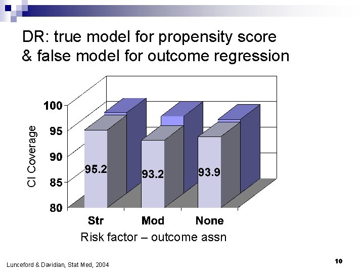
CI Coverage DR: true model for propensity score & false model for outcome regression Risk factor – outcome assn Lunceford & Davidian, Stat Med, 2004 10

Doubly robust (DR) estimation from 30, 000 feet Robins & colleagues recognized the doubly robust property in mid-90’s n Combines standardization (or reweighting) with regression n Part of the family of methods that includes propensity scores and inverse probability weighting n 11

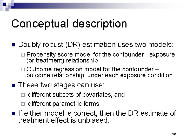
Conceptual description n Doubly robust (DR) estimation uses two models: ¨ Propensity score model for the confounder - exposure (or treatment) relationship ¨ Outcome regression model for the confounder – outcome relationship, under each exposure condition n These two stages can use: different subsets of covariates, and ¨ different parametric forms. ¨ n If either model is correct, then the DR estimate of treatment effect is unbiased. 12

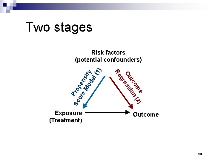
Two stages e ) om (2 tc ion Ou ess gr Exposure (Treatment) Re Sc Pro or pe e M ns od ity el (1) Risk factors (potential confounders) Outcome 13

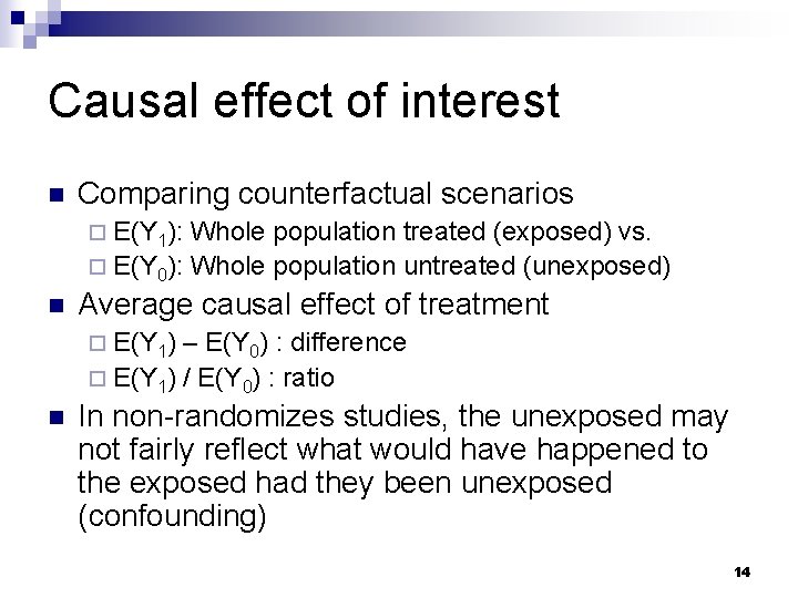
Causal effect of interest n Comparing counterfactual scenarios ¨ E(Y 1): Whole population treated (exposed) vs. ¨ E(Y 0): Whole population untreated (unexposed) n Average causal effect of treatment ¨ E(Y 1) – E(Y 0) : difference ¨ E(Y 1) / E(Y 0) : ratio n In non-randomizes studies, the unexposed may not fairly reflect what would have happened to the exposed had they been unexposed (confounding) 14

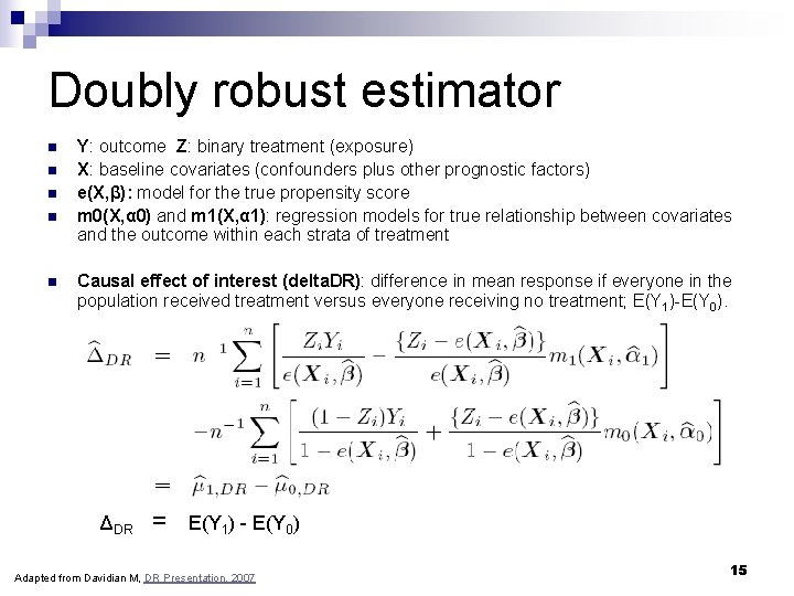
Doubly robust estimator n n n Y: outcome Z: binary treatment (exposure) X: baseline covariates (confounders plus other prognostic factors) e(X, β): model for the true propensity score m 0(X, α 0) and m 1(X, α 1): regression models for true relationship between covariates and the outcome within each strata of treatment Causal effect of interest (delta. DR): difference in mean response if everyone in the population received treatment versus everyone receiving no treatment; E(Y 1)-E(Y 0). ΔDR = E(Y 1) - E(Y 0) Adapted from Davidian M, DR Presentation, 2007 15

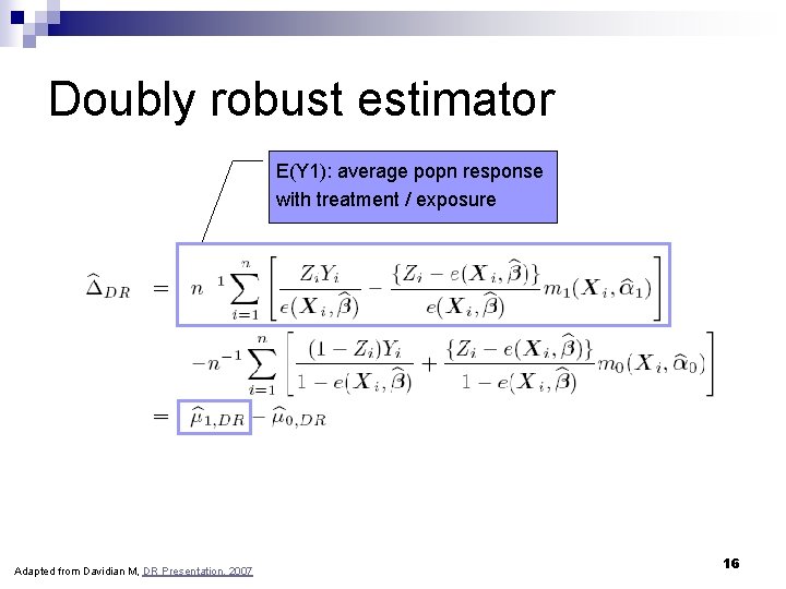
Doubly robust estimator E(Y 1): average popn response with treatment / exposure Adapted from Davidian M, DR Presentation, 2007 16

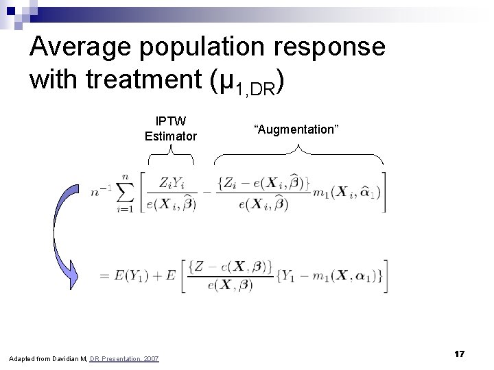
Average population response with treatment (μ 1, DR) IPTW Estimator Adapted from Davidian M, DR Presentation, 2007 “Augmentation” 17

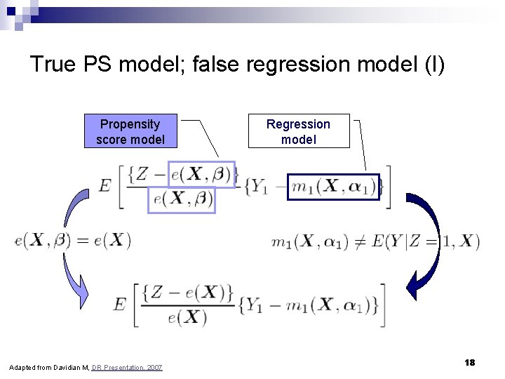
True PS model; false regression model (I) Propensity score model Adapted from Davidian M, DR Presentation, 2007 Regression model 18

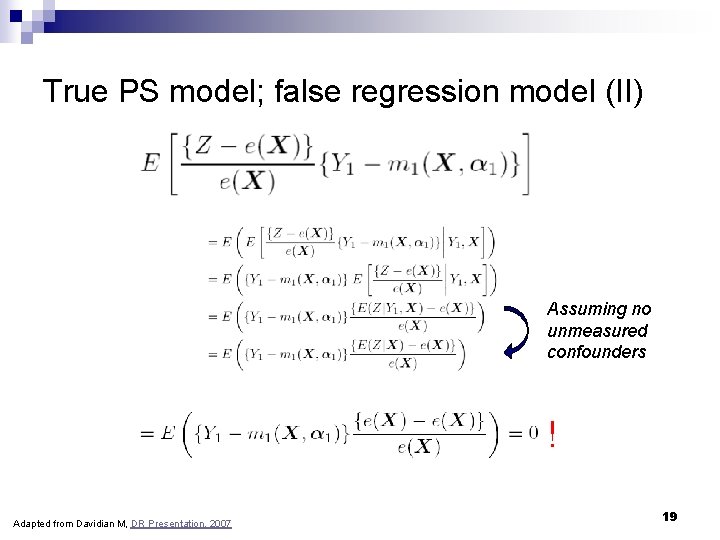
True PS model; false regression model (II) Assuming no unmeasured confounders ! Adapted from Davidian M, DR Presentation, 2007 19

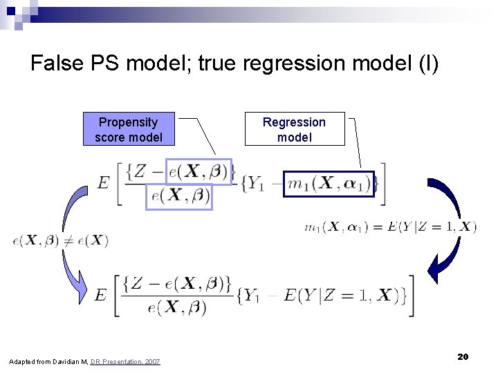
False PS model; true regression model (I) Propensity score model Adapted from Davidian M, DR Presentation, 2007 Regression model 20

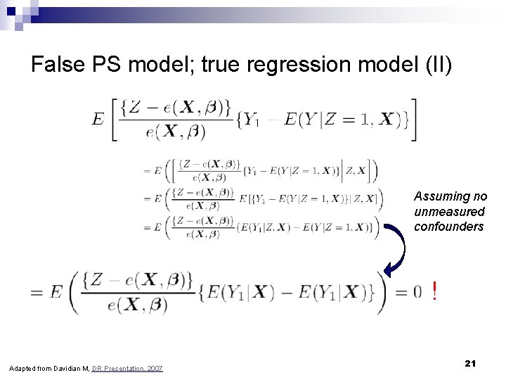
False PS model; true regression model (II) Assuming no unmeasured confounders ! Adapted from Davidian M, DR Presentation, 2007 21

Overly simplified statistics ΔDR = [E(Y 1) + junk] - [E(Y 0) + junk] Where junk = 0 if either the propensity score or the regression model is true… ΔDR = E(Y 1) - E(Y 0) Adapted from Davidian M, DR Presentation, 2007 22

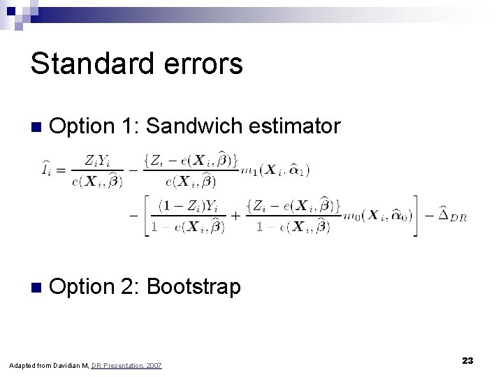
Standard errors n Option 1: Sandwich estimator n Option 2: Bootstrap Adapted from Davidian M, DR Presentation, 2007 23

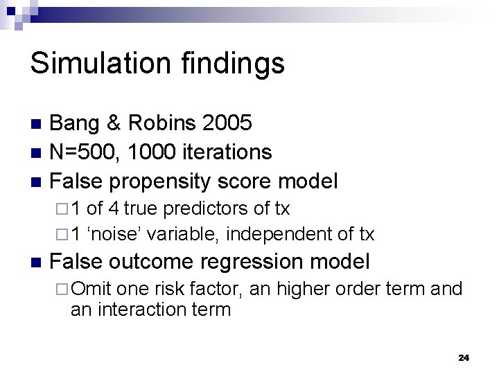
Simulation findings Bang & Robins 2005 n N=500, 1000 iterations n False propensity score model n ¨ 1 of 4 true predictors of tx ¨ 1 ‘noise’ variable, independent of tx n False outcome regression model ¨ Omit one risk factor, an higher order term and an interaction term 24

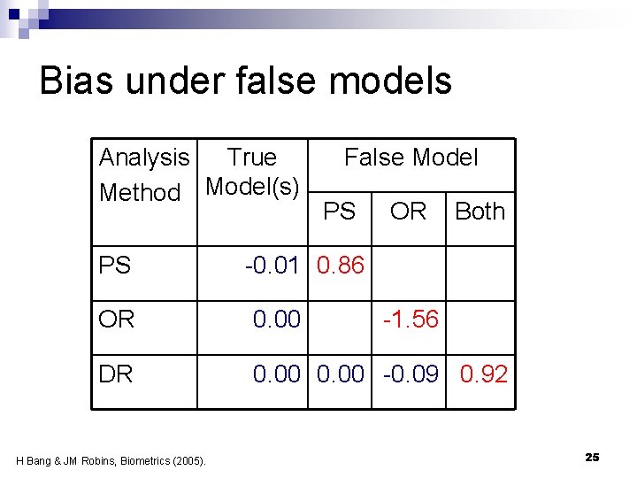
Bias under false models Analysis True Method Model(s) PS False Model PS OR Both -0. 01 0. 86 OR 0. 00 DR 0. 00 -0. 09 0. 92 H Bang & JM Robins, Biometrics (2005). -1. 56 25

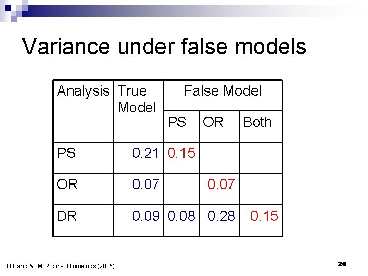
Variance under false models Analysis True Model False Model PS OR PS 0. 21 0. 15 OR 0. 07 DR 0. 09 0. 08 0. 28 H Bang & JM Robins, Biometrics (2005). Both 0. 07 0. 15 26

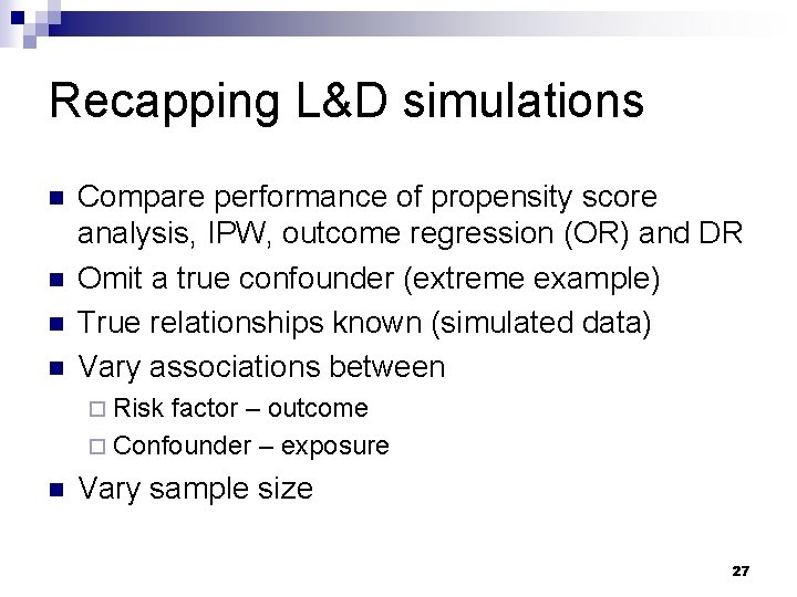
Recapping L&D simulations n n Compare performance of propensity score analysis, IPW, outcome regression (OR) and DR Omit a true confounder (extreme example) True relationships known (simulated data) Vary associations between ¨ Risk factor – outcome ¨ Confounder – exposure n Vary sample size 27

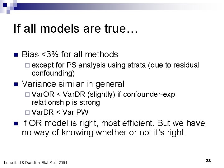
If all models are true… n Bias <3% for all methods ¨ except for PS analysis using strata (due to residual confounding) n Variance similar in general ¨ Var. OR < Var. DR (slightly) if confounder-exp relationship is strong ¨ Var. DR < Var. IPW n If OR model is right, most efficient. But we have no way of knowing whether or not it’s right. Lunceford & Davidian, Stat Med, 2004 28

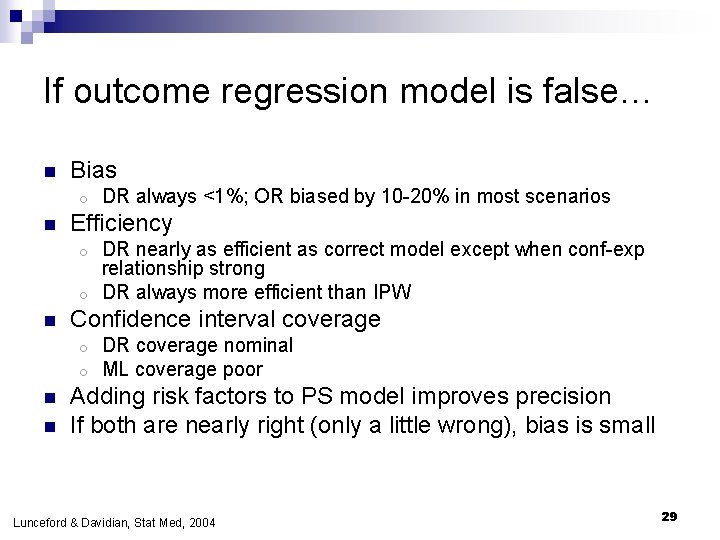
If outcome regression model is false… n Bias o n DR always <1%; OR biased by 10 -20% in most scenarios Efficiency DR nearly as efficient as correct model except when conf-exp relationship strong o DR always more efficient than IPW o n Confidence interval coverage o o n n DR coverage nominal ML coverage poor Adding risk factors to PS model improves precision If both are nearly right (only a little wrong), bias is small Lunceford & Davidian, Stat Med, 2004 29

Discussion n If method offers some protection against model misspecification, why isn’t it being used by pharmacoepidemiologists? 30

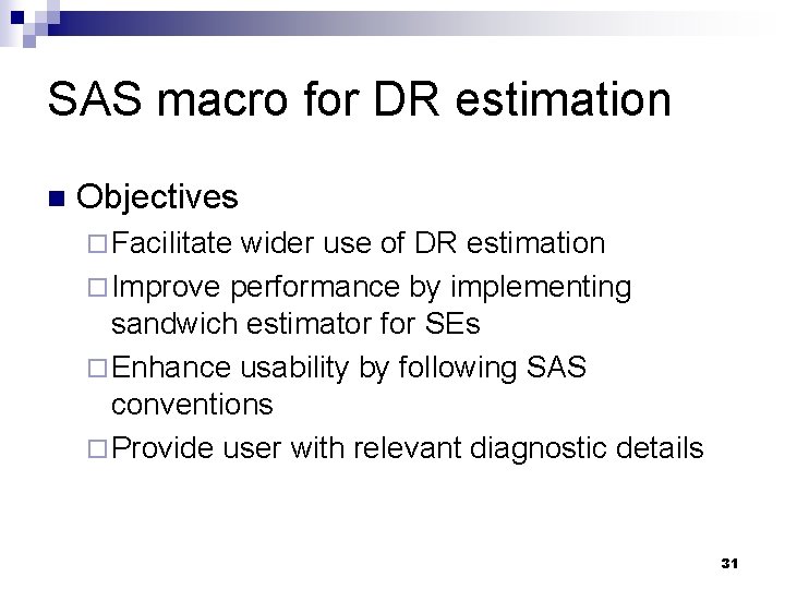
SAS macro for DR estimation n Objectives ¨ Facilitate wider use of DR estimation ¨ Improve performance by implementing sandwich estimator for SEs ¨ Enhance usability by following SAS conventions ¨ Provide user with relevant diagnostic details 31

http: //www. harryguess. unc. edu SAS macro for doubly robust estimation including documentation Dataset for sample analyses (1. 7 MB, optional) 32

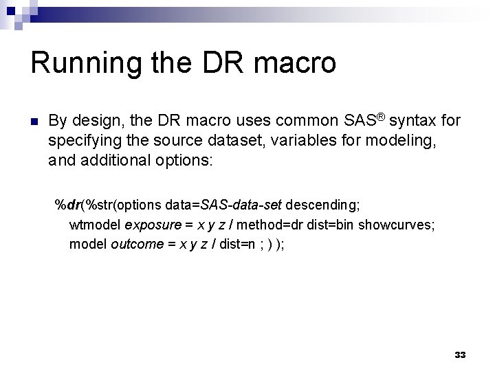
Running the DR macro n By design, the DR macro uses common SAS® syntax for specifying the source dataset, variables for modeling, and additional options: %dr(%str(options data=SAS-data-set descending; wtmodel exposure = x y z / method=dr dist=bin showcurves; model outcome = x y z / dist=n ; ) ); 33

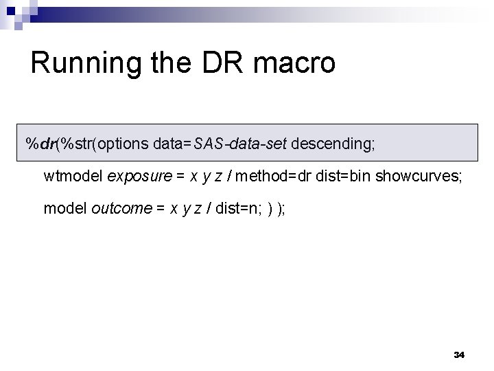
Running the DR macro %dr(%str(options data=SAS-data-set descending; wtmodel exposure = x y z / method=dr dist=bin showcurves; model outcome = x y z / dist=n; ) ); 34

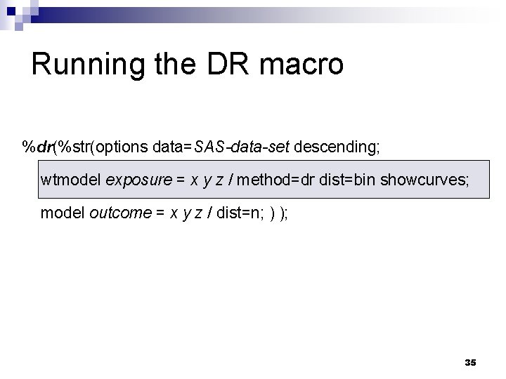
Running the DR macro %dr(%str(options data=SAS-data-set descending; wtmodel exposure = x y z / method=dr dist=bin showcurves; model outcome = x y z / dist=n; ) ); 35

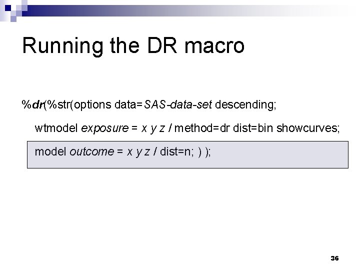
Running the DR macro %dr(%str(options data=SAS-data-set descending; wtmodel exposure = x y z / method=dr dist=bin showcurves; model outcome = x y z / dist=n; ) ); 36

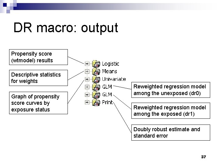
DR macro: output Propensity score (wtmodel) results Descriptive statistics for weights Graph of propensity score curves by exposure status Reweighted regression model among the unexposed (dr 0) Reweighted regression model among the exposed (dr 1) Doubly robust estimate and standard error 37

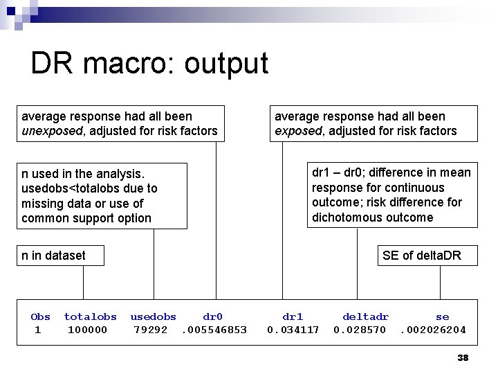
DR macro: output average response had all been unexposed, adjusted for risk factors n used in the analysis. usedobs<totalobs due to missing data or use of common support option average response had all been exposed, adjusted for risk factors dr 1 – dr 0; difference in mean response for continuous outcome; risk difference for dichotomous outcome n in dataset Obs 1 totalobs 100000 SE of delta. DR usedobs dr 0 79292. 005546853 dr 1 0. 034117 deltadr se 0. 028570. 002026204 38

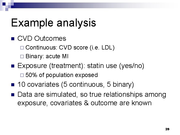
Example analysis n CVD Outcomes ¨ Continuous: CVD score (i. e. LDL) ¨ Binary: acute MI n Exposure (treatment): statin use (yes/no) ¨ 50% n n of population exposed 10 covariates (5 continuous, 5 binary) Data are simulated, so true relationships among exposure, covariates & outcome are known 39

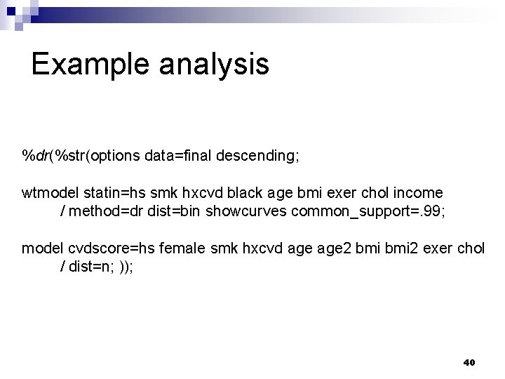
Example analysis %dr(%str(options data=final descending; wtmodel statin=hs smk hxcvd black age bmi exer chol income / method=dr dist=bin showcurves common_support=. 99; model cvdscore=hs female smk hxcvd age 2 bmi 2 exer chol / dist=n; )); 40

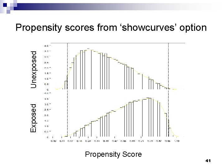
Exposed Unexposed Propensity scores from ‘showcurves’ option Propensity Score 41

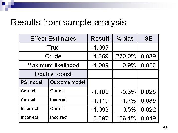
Results from sample analysis Effect Estimates True Crude Maximum likelihood Doubly robust PS model Outcome model Correct Incorrect Result -1. 099 1. 869 -1. 089 %bias SE 270. 0% 0. 089 0. 9% 0. 023 -1. 102 -1. 117 -1. 093 0. 397 -0. 3% -1. 7% 0. 5% 136. 1% 0. 025 0. 089 0. 022 0. 049 42

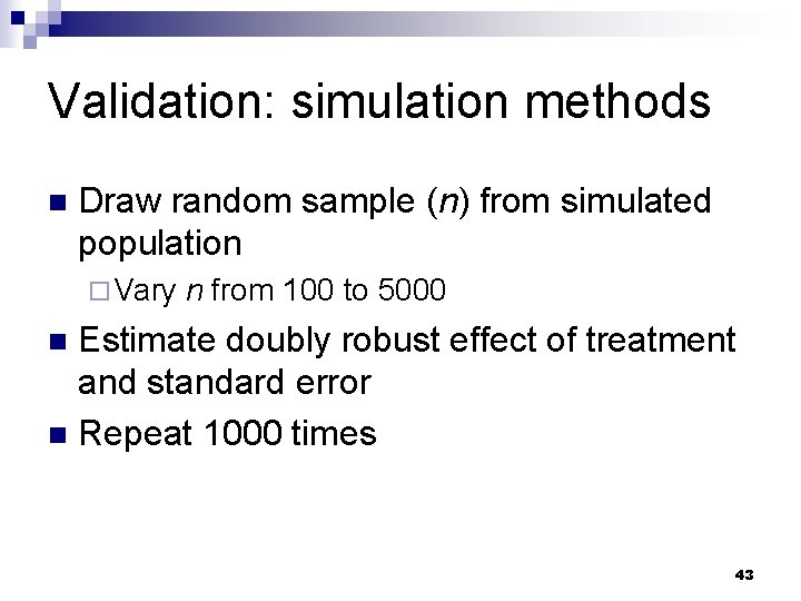
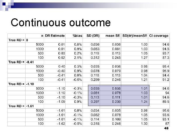
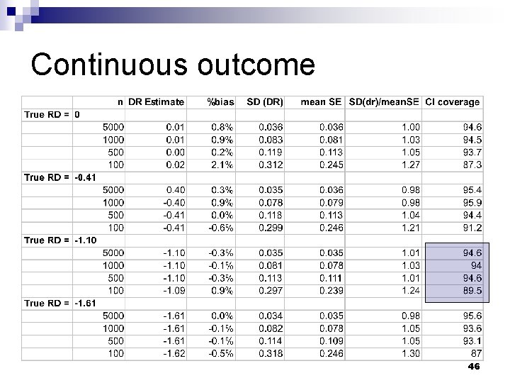
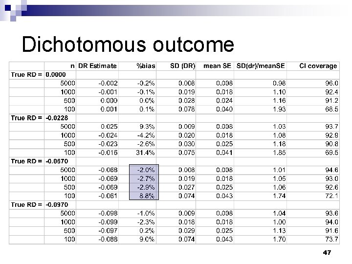
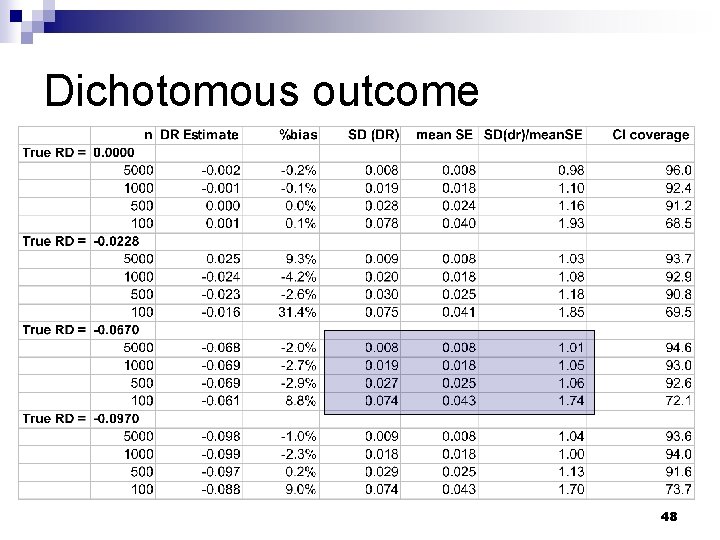
Validation: simulation methods n Draw random sample (n) from simulated population ¨ Vary n from 100 to 5000 Estimate doubly robust effect of treatment and standard error n Repeat 1000 times n 43

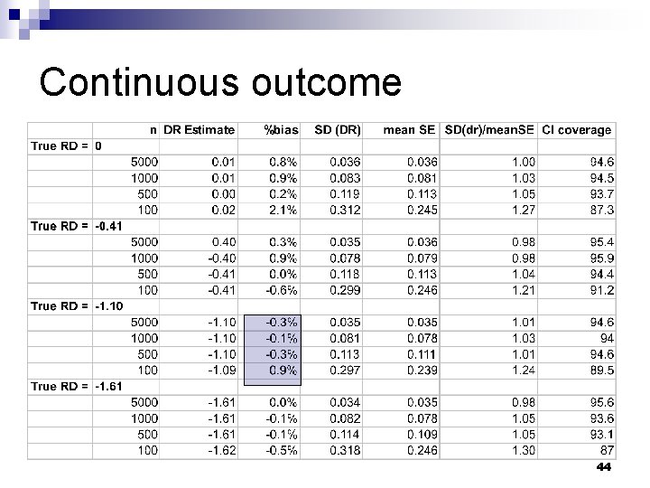
Continuous outcome 44

Continuous outcome 45

Continuous outcome 46

Dichotomous outcome 47

Dichotomous outcome 48

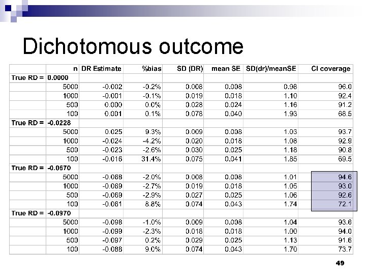
Dichotomous outcome 49

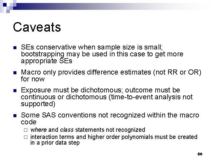
Caveats n SEs conservative when sample size is small; bootstrapping may be used in this case to get more appropriate SEs n Macro only provides difference estimates (not RR or OR) for now n Exposure must be dichotomous; outcome must be continuous or dichotomous (time-to-event analysis not supported) n Some SAS conventions not recognized within the macro code ¨ ¨ where and class statements not recognized interaction terms and higher order polynomials must be created in a prior data step 50

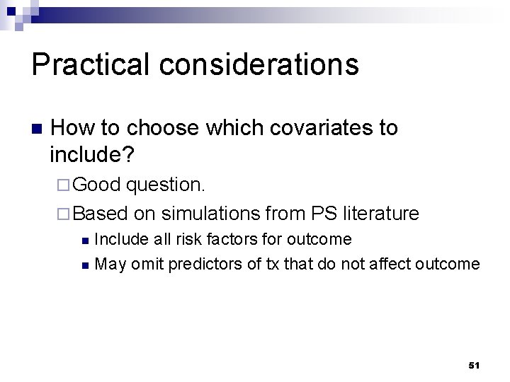
Practical considerations n How to choose which covariates to include? ¨ Good question. ¨ Based on simulations from PS literature Include all risk factors for outcome n May omit predictors of tx that do not affect outcome n 51

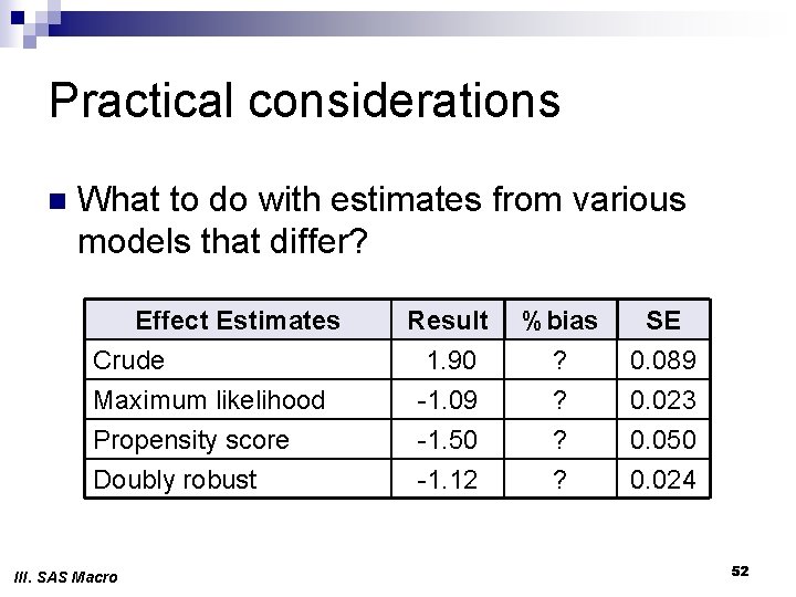
Practical considerations n What to do with estimates from various models that differ? Effect Estimates Crude Maximum likelihood Propensity score Doubly robust III. SAS Macro Result 1. 90 -1. 09 -1. 50 -1. 12 %bias ? ? SE 0. 089 0. 023 0. 050 0. 024 52

Practical considerations n What sort of diagnostics should be checked? ¨ Potentially influential obs with extreme PS values n ‘common_support’ option in SAS macro ¨ Distribution of PS scores stratified by treatment / exposure group n ‘showcurves’ option in SAS macro 53

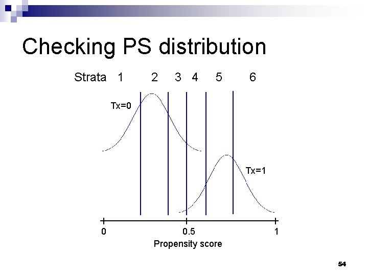
Checking PS distribution Strata 1 2 3 4 5 6 Tx=0 Tx=1 0 0. 5 Propensity score 1 54

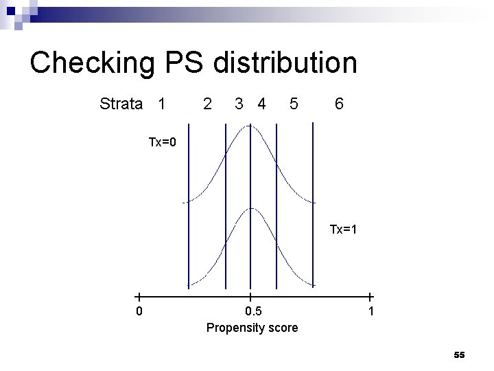
Checking PS distribution Strata 1 2 3 4 5 6 Tx=0 Tx=1 0 0. 5 Propensity score 1 55

Checking PS distribution Strata 1 2 3 4 5 6 Tx=0 Tx=1 0 0. 5 Propensity score 1 56

Limitations n DR estimation is not a panacea for unmeasured confounding. ¨ n Recall- ‘junk’ only reduces to 0 with assumption of no unmeasured confounders One of the models must be correct for the estimator to be unbiased ¨ Bang & Robins suggest that it will be minimally biased if both models are nearly right… n Standard errors tend to be slightly larger compared to a single correctly specified regression model n Explaining DR estimation in your methods section could be interesting… 57

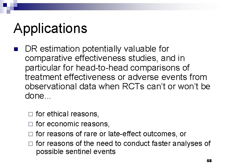
Applications n DR estimation potentially valuable for comparative effectiveness studies, and in particular for head-to-head comparisons of treatment effectiveness or adverse events from observational data when RCTs can’t or won’t be done. . . for ethical reasons, ¨ for economic reasons, ¨ for reasons of rare or late-effect outcomes, or ¨ for reasons of the need to conduct faster analyses of possible sentinel events ¨ 58

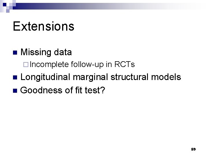
Extensions n Missing data ¨ Incomplete follow-up in RCTs Longitudinal marginal structural models n Goodness of fit test? n 59

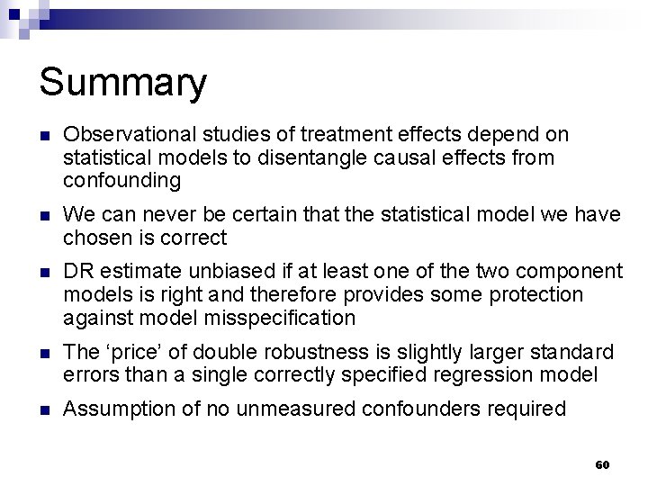
Summary n Observational studies of treatment effects depend on statistical models to disentangle causal effects from confounding n We can never be certain that the statistical model we have chosen is correct n DR estimate unbiased if at least one of the two component models is right and therefore provides some protection against model misspecification n The ‘price’ of double robustness is slightly larger standard errors than a single correctly specified regression model n Assumption of no unmeasured confounders required 60

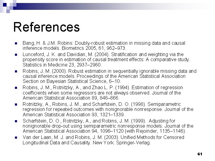
References n n n n Bang, H. & J. M. Robins: Doubly-robust estimation in missing data and causal inference models. Biometrics 2005, 61, 962– 973. Lunceford, J. K. and Davidian, M. (2004). Stratification and weighting via the propensity score in estimation of causal treatment effects: A comparative study. Statistics in Medicine 23, 2937– 2960. Robins, J. M. (2000). Robust estimation in sequentially ignorable missing data and causal inference models. Proceedings of the American Statistical Association Section on Bayesian Statistical Science, 6– 10. Robins, J. M. , Rotnitzky, A. , and Zhao L. P. (1994). Estimation of regression coefficients when some regressors are not always observed. Journal of the American Statistical Association 89, 846– 866. Rotnitzky, A. , Robins, J. M. , and Scharfstein, D. O. (1998). Semiparametric regression for repeated outcomes with nonignorable nonresponse. Journal of the American Statistical Association 93, 1321– 1339. Scharfstein, D. O. , Rotnitzky, A. , and Robins, J. M. (1999). Adjusting for nonignorable drop-out using semiparametric nonresponse models. Journal of the American Statistical Association 94, 1096– 1120 (with Rejoinder, 1135– 1146). Van der Laan, M. J. and Robins, J. M. (2003). Unified Methods for Censored Longitudinal Data and Causality. New York: Springer-Verlag. 61

Acknowledgements Collaborators on the development of the SAS macro: n Chris Wiesen, Ph. D, Odum Institute for Research in Social Science, University of North Carolina, Chapel Hill, NC n Daniel Westreich, MSPH, Department of Epidemiology, University of North Carolina, Chapel Hill, NC n Marie Davidian, Ph. D, Department of Statistics, North Carolina State University, Raleigh, NC 62

Acknowledgements (II) n Agency for Healthcare Research and Quality Supplemental Award to the UNC CERTs (U 18 HS 10397 -07 S 1) n UNC/GSK Center for Excellence in Pharmacoepidemiology and Public Health n Kevin Anstrom, Lesley Curtis, Brad Hammill, and Rex Edwards from the Duke CERTs team for valuable feedback on the alpha version. n Thanks to students from UNC’s EPID 369/730, a causal modeling course, for valuable feedback on the beta version. n Presented in memory of Harry Guess, MD, Ph. D, 1940 -2006, who co-authored the initial proposal to develop a SAS macro for doubly robust estimation. 63

Contact Information Michele Jonsson Funk, Ph. D Research Assistant Professor Department of Epidemiology University of North Carolina Chapel Hill NC 27599 -7521 mfunk@unc. edu 919 -966 -8431 (ph) 919 -843 -3120 (fax) http: //www. harryguess. unc. edu 64

Questions & Discussion 65