A Visual Programming Language for Biological Processes Andrew

A Visual Programming Language for Biological Processes Andrew Phillips with Luca Cardelli Microsoft Research, Cambridge UK
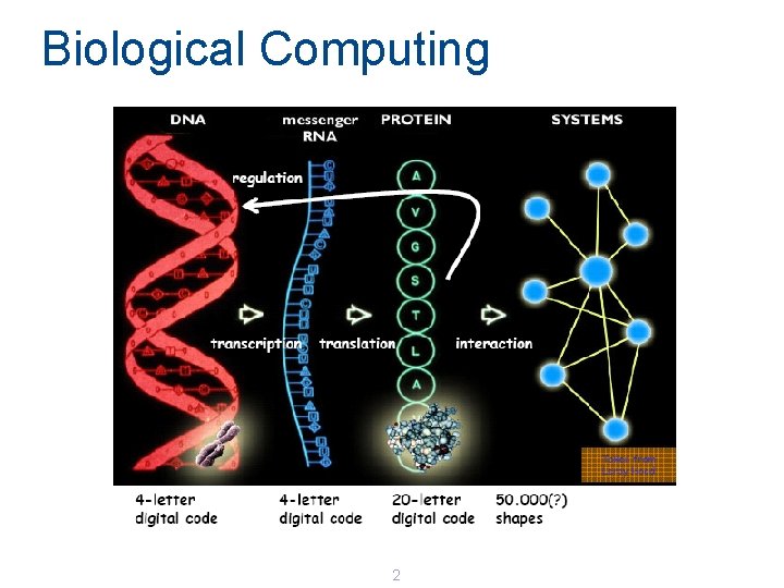
Biological Computing 2
Systems Biology The Human Genome project: Map out the complete genetic code in humans To unravel the mysteries of how the human body functions The code raised many more questions than answers Systems Biology: Understand predict the behaviour of biological systems Two complementary approaches: Look at experimental results and infer system properties Build detailed models of systems and test these in the lab Biological Modelling: Conduct virtual experiments, saving time and resources Clarify key mechanisms of how a biological system functions Beginning to play a role in understanding disease
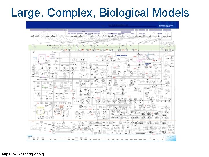
Large, Complex, Biological Models http: //www. celldesigner. org
Biological Programming Complex Models: Difficult to understand, maintain and extend Hundreds of reactions, soon to be tens of thousands Would not write a program as a list of 10000 instructions Modularity: Need a way of decomposing a model into building blocks Not your average computer programs Massive parallelism, each instruction has a certain probability Suggests a need for a biological programming language. . .
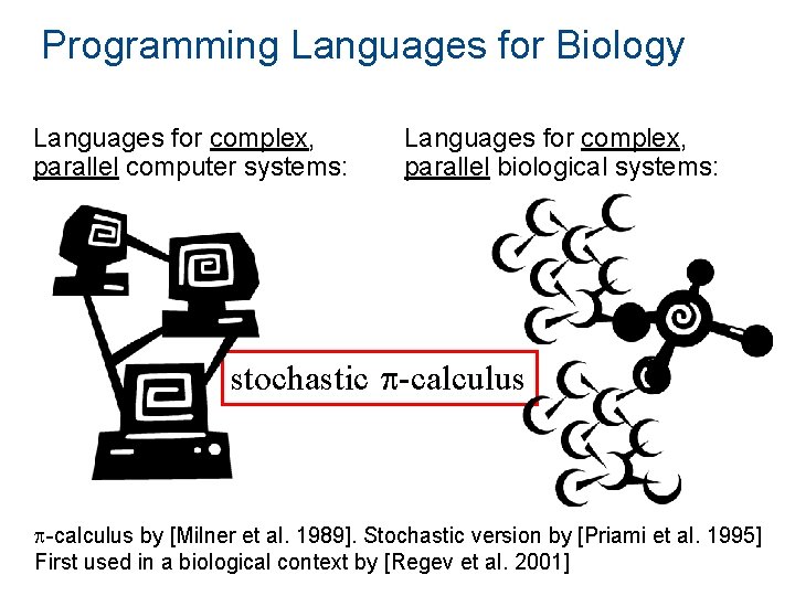
Programming Languages for Biology Languages for complex, parallel computer systems: Languages for complex, parallel biological systems: stochastic p-calculus by [Milner et al. 1989]. Stochastic version by [Priami et al. 1995] First used in a biological context by [Regev et al. 2001]
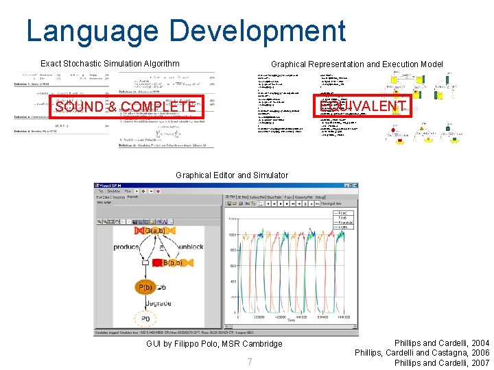
Language Development Exact Stochastic Simulation Algorithm Graphical Representation and Execution Model let g. Low() = delay@g_pep; (Low() | g. Low()) and Low()= ( new low@u. Low: chan do !pep(low); ? low; Low() or delay@d_pep ) let g. Med() = delay@g_pep; (Med() | g. Med()) and Med()= ( new med@u. Med: chan do !pep(med); ? med; Med() or delay@d_pep ) let g. High() = delay@g_pep; (High() | g. High()) and High()= ( new high@u. High: chan do !pep(high); ? high; High() or delay@d_pep ) let g. MHC() = delay@g_MHC; (g. MHC() | MHCo() ) and g. TPN() = delay@g_TPN; ( g. TPN() | TPN() ) SOUND & COMPLETE and TPN()= ( new u. T@unbind_TPN: chan do !tpn(u. T); ? u. T; TPN() or delay@degrade_TPN ) and MHCo()= do ? pep(u); MHCc_pep(u) or ? tpn(u. T); MHCo_TPN(u. T) or delay@degrade_MHCo and MHCc_pep(u: chan) = do delay@egress; MHCe_pep(u) or !u; MHCo() and MHCe_pep(u: chan) = delay@degrade_MHCe EQUIVALENT and MHCo_TPN(u. T: chan)= do ? pep(u)*a; MHCc_TPN_pep(u, u. T) or !u. T*v; MHCo() and MHCc_TPN_pep(u: chan, u. T: chan)= do !u. T; MHCc_pep(u) or !u*q; MHCo_TPN(u. T) Graphical Editor and Simulator GUI by Filippo Polo, MSR Cambridge 7 Phillips and Cardelli, 2004 Phillips, Cardelli and Castagna, 2006 Phillips and Cardelli, 2007

SPi. M: Stochastic p for Biology A variant of stochastic p calculus Supports expressive power of p Graphical syntax and semantics Biological constructs, e. g. complexation Efficient implementation 8
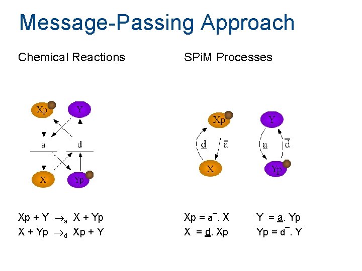
Message-Passing Approach Chemical Reactions Xp + Y a X + Yp d Xp + Y SPi. M Processes _ Xp = a. X X = d. Xp Y = a. Yp _ Yp = d. Y
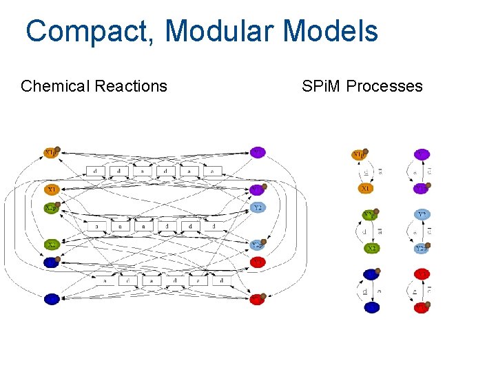
Compact, Modular Models Chemical Reactions SPi. M Processes
![EGFR Model [Hornberg et. al 2005] 11 EGFR Model [Hornberg et. al 2005] 11](http://slidetodoc.com/presentation_image_h2/53d5aaf19256564706e65910e40b97de/image-11.jpg)
EGFR Model [Hornberg et. al 2005] 11
![EGFR Model [Hornberg et. al 2005] 12 EGFR Model [Hornberg et. al 2005] 12](http://slidetodoc.com/presentation_image_h2/53d5aaf19256564706e65910e40b97de/image-12.jpg)
EGFR Model [Hornberg et. al 2005] 12
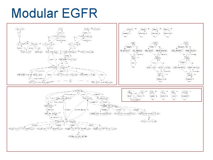
Modular EGFR
Outline Basic Examples Gene Networks C. elegans Development Immune System Modelling 14
Basic SPi. M Examples Protein Production Protein Interaction Protein Binding
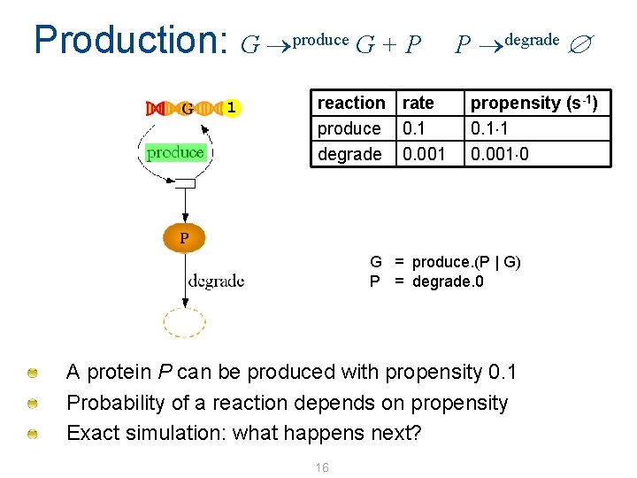
Production: G produce G + P 1 reaction rate produce 0. 1 degrade 0. 001 P degrade propensity (s-1) 0. 1 1 0. 001 0 G = produce. (P | G) P = degrade. 0 A protein P can be produced with propensity 0. 1 Probability of a reaction depends on propensity Exact simulation: what happens next? 16
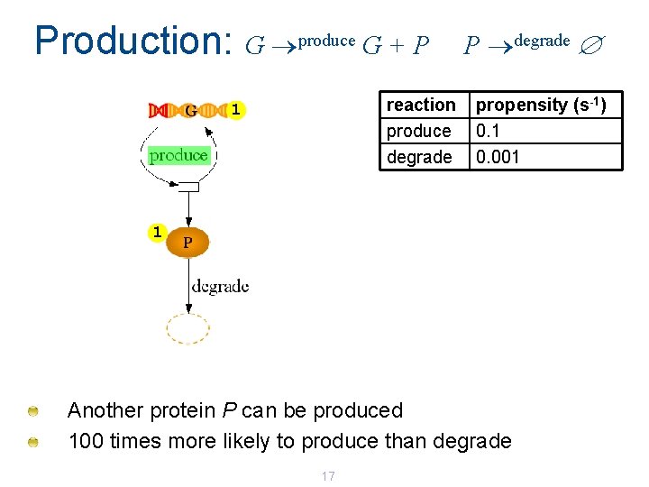
Production: G produce G + P reaction produce degrade 1 P degrade propensity (s-1) 0. 1 0. 001 1 Another protein P can be produced 100 times more likely to produce than degrade 17
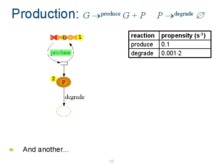
Production: G produce G + P reaction produce degrade 1 2 And another. . . 18 P degrade propensity (s-1) 0. 1 0. 001 2
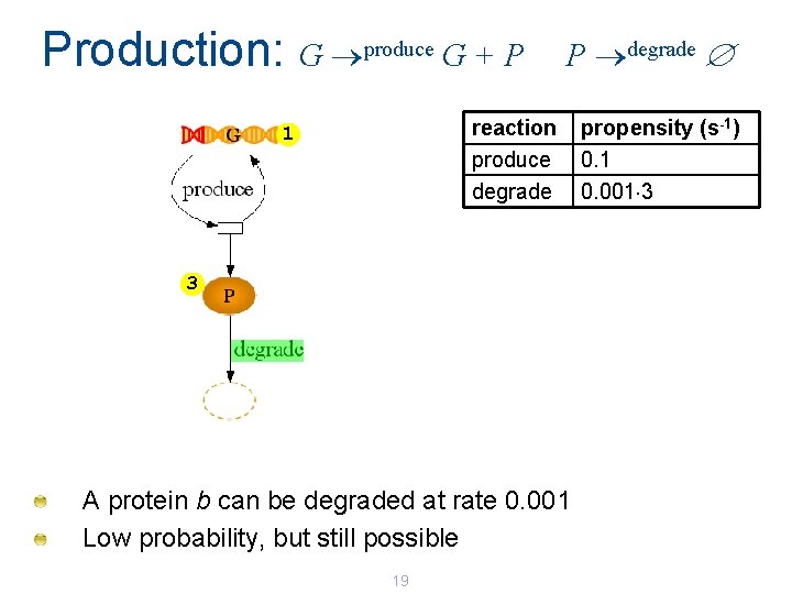
Production: G produce G + P P degrade reaction produce degrade 1 3 A protein b can be degraded at rate 0. 001 Low probability, but still possible 19 propensity (s-1) 0. 1 0. 001 3
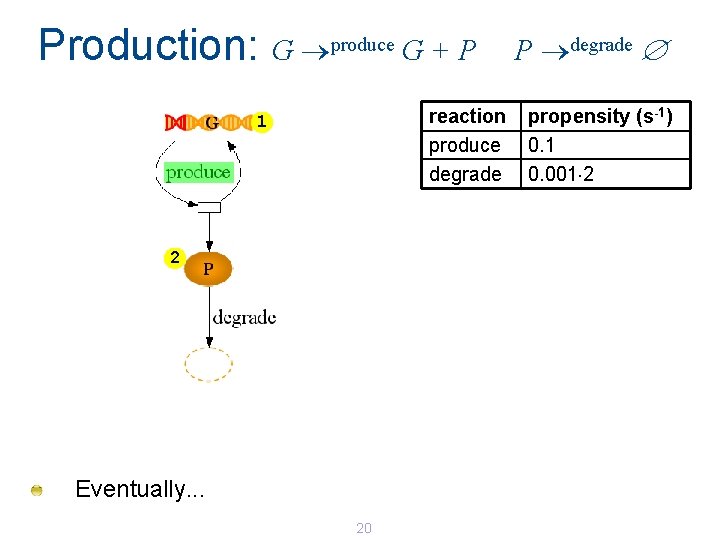
Production: G produce G + P reaction produce degrade 1 2 Eventually. . . 20 P degrade propensity (s-1) 0. 1 0. 001 2
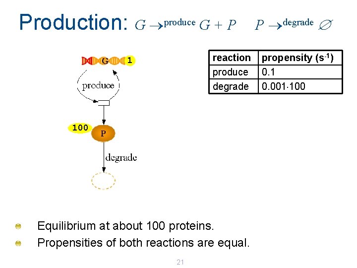
Production: G produce G + P reaction produce degrade 1 100 Equilibrium at about 100 proteins. Propensities of both reactions are equal. 21 P degrade propensity (s-1) 0. 1 0. 001 100
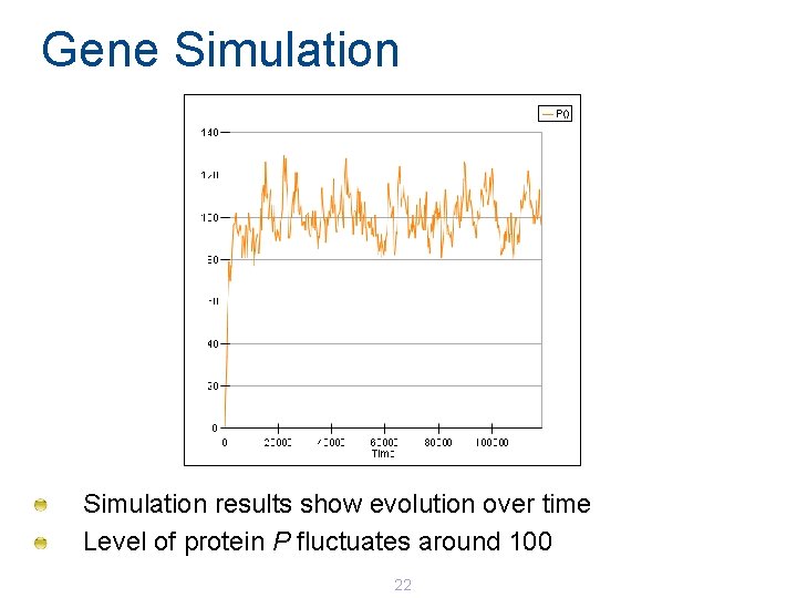
Gene Simulation results show evolution over time Level of protein P fluctuates around 100 22
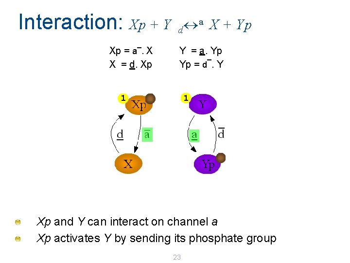
Interaction: Xp + Y _ Xp = a. X X = d. Xp a X + Yp d Y = a. Yp _ Yp = d. Y 1 1 Xp and Y can interact on channel a Xp activates Y by sending its phosphate group 23
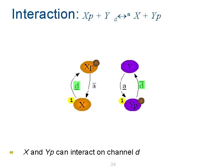
Interaction: Xp + Y a X + Yp d 1 1 X and Yp can interact on channel d 24
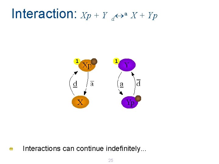
Interaction: Xp + Y a X + Yp d 1 1 Interactions can continue indefinitely. . . 25
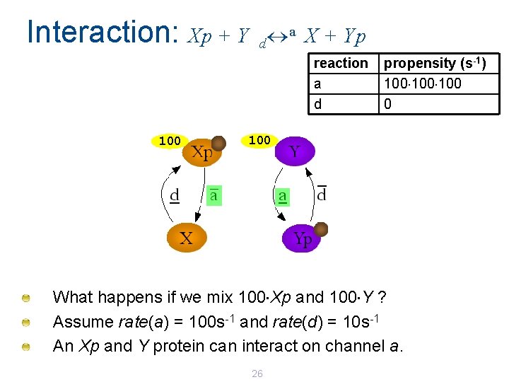
Interaction: Xp + Y a X + Yp d reaction a d 100 propensity (s-1) 100 100 What happens if we mix 100 Xp and 100 Y ? Assume rate(a) = 100 s-1 and rate(d) = 10 s-1 An Xp and Y protein can interact on channel a. 26
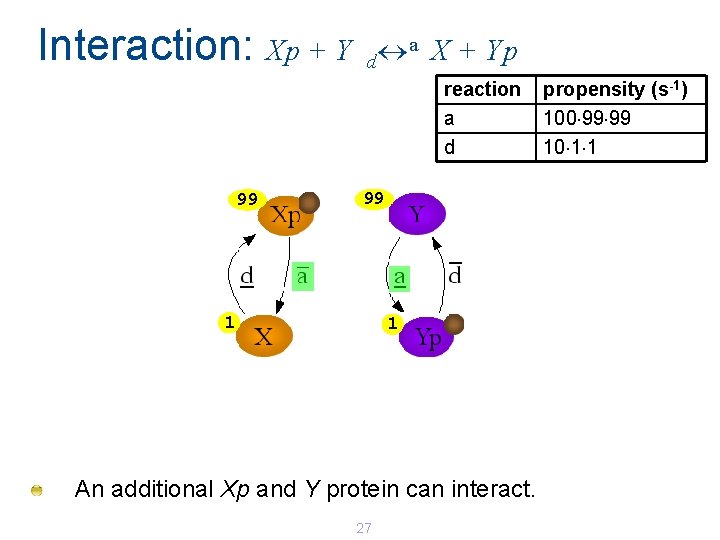
Interaction: Xp + Y a X + Yp d reaction a d 99 99 1 1 An additional Xp and Y protein can interact. 27 propensity (s-1) 100 99 99 10 1 1
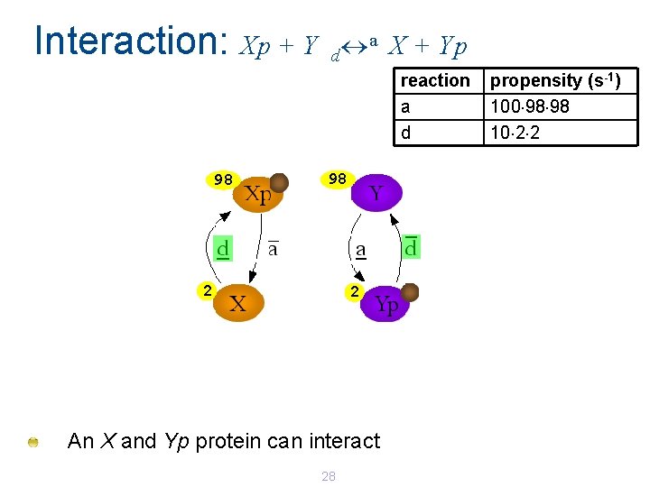
Interaction: Xp + Y a X + Yp d reaction a d 98 98 2 2 An X and Yp protein can interact 28 propensity (s-1) 100 98 98 10 2 2
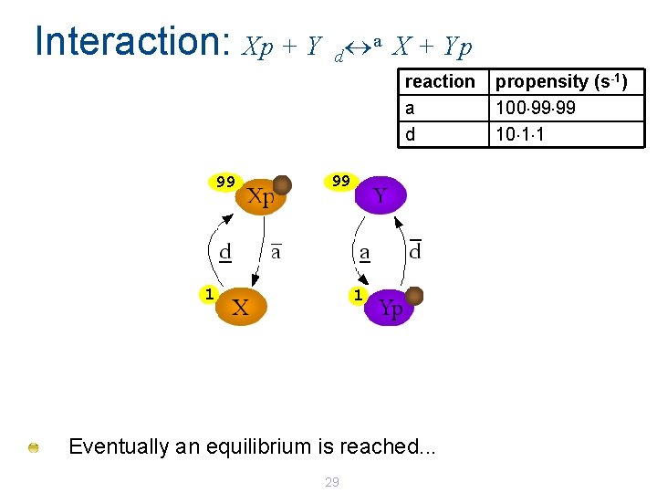
Interaction: Xp + Y a X + Yp d reaction a d 99 99 1 1 Eventually an equilibrium is reached. . . 29 propensity (s-1) 100 99 99 10 1 1
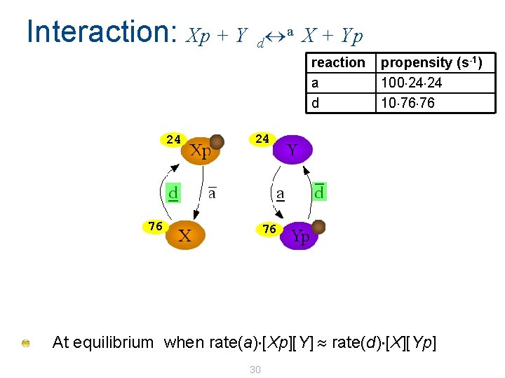
Interaction: Xp + Y a X + Yp d reaction a d 24 propensity (s-1) 100 24 24 10 76 76 24 76 76 At equilibrium when rate(a) [Xp][Y] rate(d) [X][Yp] 30
![Interaction: Xp + Y a X + Yp d At equilibrium: 100 s-1 [Xp][Y] Interaction: Xp + Y a X + Yp d At equilibrium: 100 s-1 [Xp][Y]](http://slidetodoc.com/presentation_image_h2/53d5aaf19256564706e65910e40b97de/image-31.jpg)
Interaction: Xp + Y a X + Yp d At equilibrium: 100 s-1 [Xp][Y] 10 s-1 [X][Yp] Approximately 24 Xp and 76 X 31
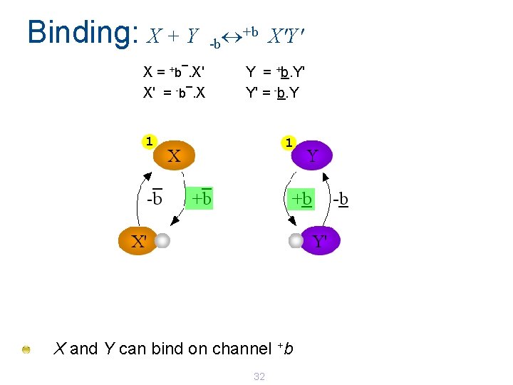
Binding: X + Y _ X=. X' _ X' = -b. X +b +b X'Y' -b Y = +b. Y' Y' = -b. Y 1 1 X and Y can bind on channel +b 32
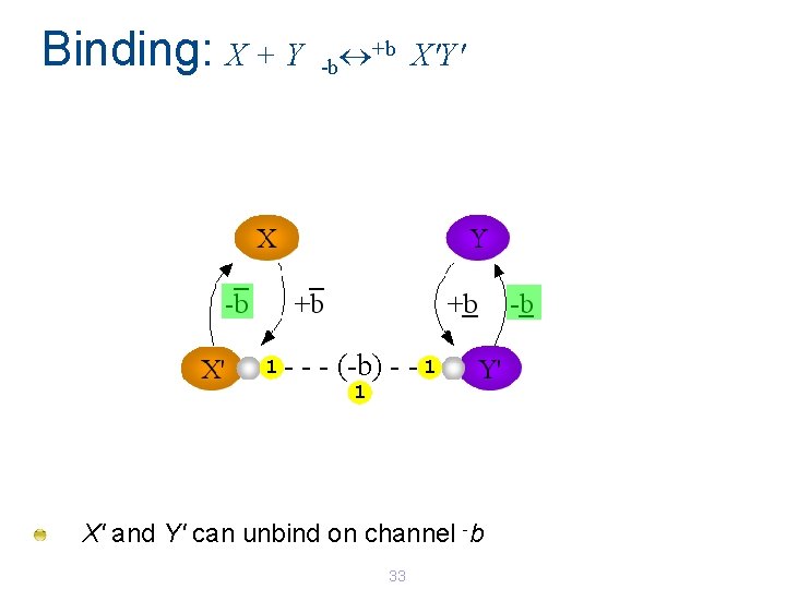
Binding: X + Y 1 - +b X'Y' -b - - (-b) - - 1 1 X' and Y' can unbind on channel -b 33
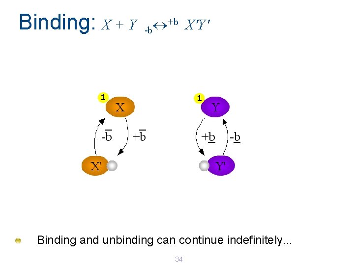
Binding: X + Y +b X'Y' -b 1 1 Binding and unbinding can continue indefinitely. . . 34
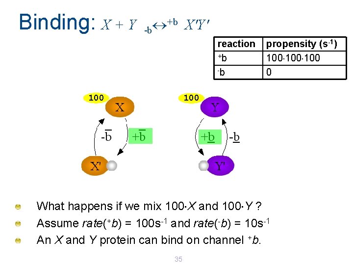
Binding: X + Y +b X'Y' -b reaction +b -b 100 propensity (s-1) 100 100 What happens if we mix 100 X and 100 Y ? Assume rate(+b) = 100 s-1 and rate(-b) = 10 s-1 An X and Y protein can bind on channel +b. 35
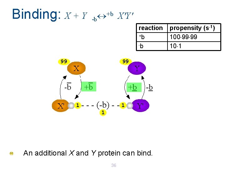
Binding: X + Y +b X'Y' -b reaction +b -b 99 99 1 - - - (-b) - - 1 1 An additional X and Y protein can bind. 36 propensity (s-1) 100 99 99 10 1
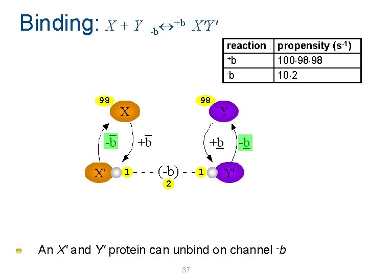
Binding: X + Y +b X'Y' -b reaction +b -b propensity (s-1) 100 98 98 10 2 98 98 1 - - - (-b) - - 1 2 An X' and Y' protein can unbind on channel -b 37
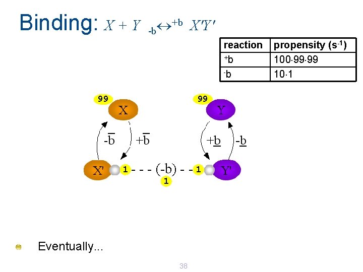
Binding: X + Y +b X'Y' -b reaction +b -b 99 99 1 - - - (-b) - - 1 1 Eventually. . . 38 propensity (s-1) 100 99 99 10 1
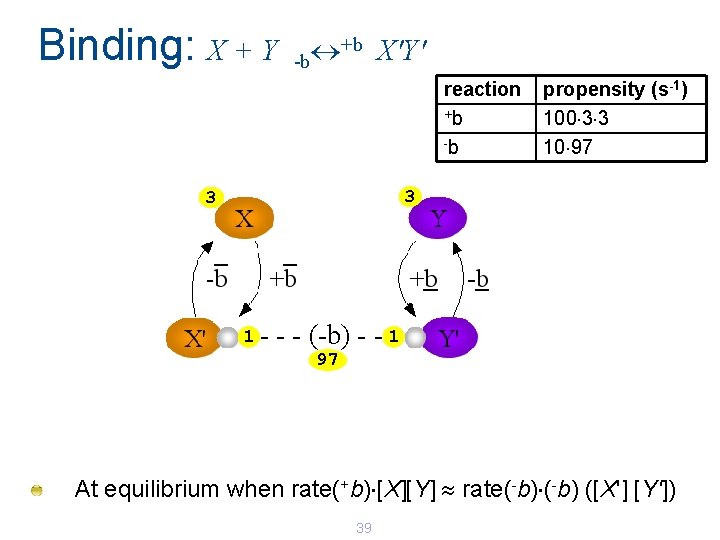
Binding: X + Y +b X'Y' -b reaction +b -b propensity (s-1) 100 3 3 10 97 3 3 1 - - - (-b) - - 1 97 At equilibrium when rate(+b) [X][Y] rate(-b) ([X'] [Y']) 39
![Binding: X + Y +b X'Y' -b At equilibrium: 100 s-1 [X][Y] = 10 Binding: X + Y +b X'Y' -b At equilibrium: 100 s-1 [X][Y] = 10](http://slidetodoc.com/presentation_image_h2/53d5aaf19256564706e65910e40b97de/image-40.jpg)
Binding: X + Y +b X'Y' -b At equilibrium: 100 s-1 [X][Y] = 10 s-1 [X'Y'] Approximately 3 X and 97 X'Y' 40
Programming Gene Networks with Luca Cardelli (MSR Cambridge) Ralf Blossey (IRI Lille)
![Repressilator [Elowitz and Leibler, 2000] A gene network engineered in live bacteria. © 2000 Repressilator [Elowitz and Leibler, 2000] A gene network engineered in live bacteria. © 2000](http://slidetodoc.com/presentation_image_h2/53d5aaf19256564706e65910e40b97de/image-42.jpg)
Repressilator [Elowitz and Leibler, 2000] A gene network engineered in live bacteria. © 2000 Elowitz, M. B. , Leibler. S. A Synthetic Oscillatory Network of Transcriptional Regulators. Nature 403: 335 -338.
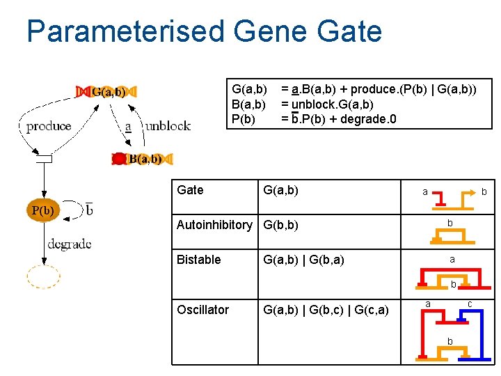
Parameterised Gene Gate G(a, b) B(a, b) P(b) Gate = a. B(a, b) + produce. (P(b) | G(a, b)) = unblock. G(a, b) = b. P(b) + degrade. 0 G(a, b) a b Autoinhibitory G(b, b) b Bistable a G(a, b) | G(b, a) b Oscillator G(a, b) | G(b, c) | G(c, a) a c b
![Repressilator [Elowitz and Leibler, 2000] Modelled as a simple combination of gene gates: G(lac, Repressilator [Elowitz and Leibler, 2000] Modelled as a simple combination of gene gates: G(lac,](http://slidetodoc.com/presentation_image_h2/53d5aaf19256564706e65910e40b97de/image-44.jpg)
Repressilator [Elowitz and Leibler, 2000] Modelled as a simple combination of gene gates: G(lac, tet) | G(tet, lambda) | G(lambda, lac) | G(tet, gfp) © 2000 Elowitz, M. B. , Leibler. S. A Synthetic Oscillatory Network of Transcriptional Regulators. Nature 403: 335 -338. lac lambda tet gfp
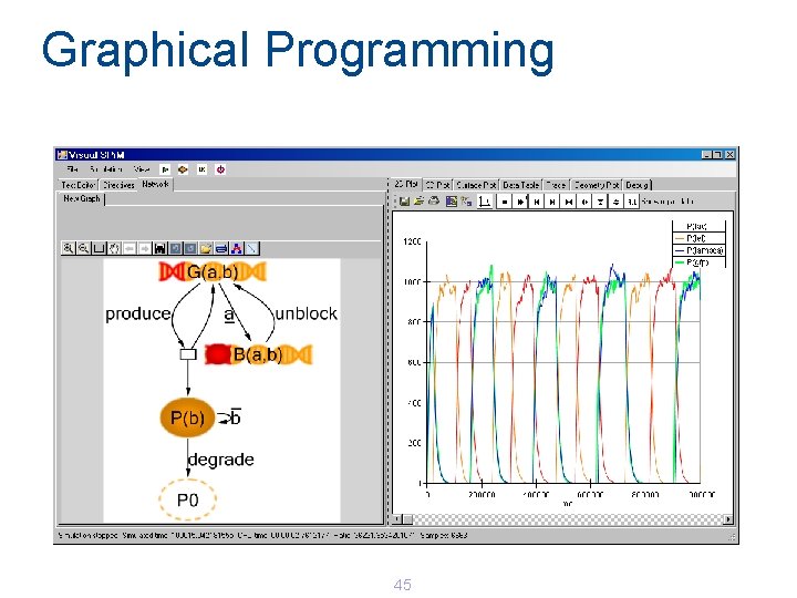
Graphical Programming 45
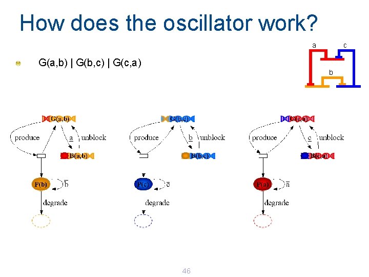
How does the oscillator work? a c G(a, b) | G(b, c) | G(c, a) b 46
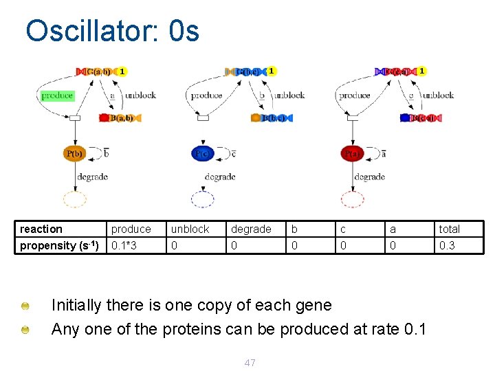
Oscillator: 0 s 1 1 1 reaction produce unblock degrade b c a total propensity (s-1) 0. 1*3 0 0 0. 3 Initially there is one copy of each gene Any one of the proteins can be produced at rate 0. 1 47
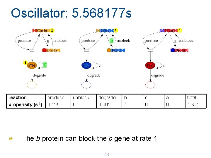
Oscillator: 5. 568177 s 1 1 reaction produce unblock degrade b c a total propensity (s-1) 0. 1*3 0 0. 001 1 0 0 1. 301 The b protein can block the c gene at rate 1 48
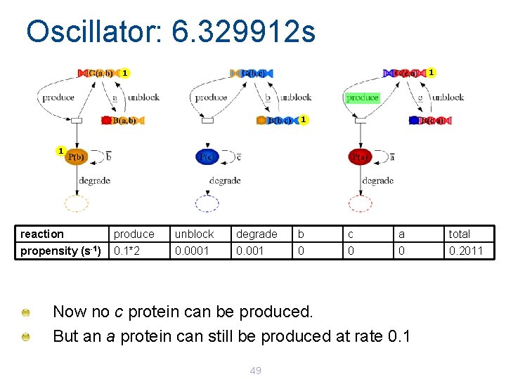
Oscillator: 6. 329912 s 1 1 reaction produce unblock degrade b c a total propensity (s-1) 0. 1*2 0. 0001 0 0. 2011 Now no c protein can be produced. But an a protein can still be produced at rate 0. 1 49
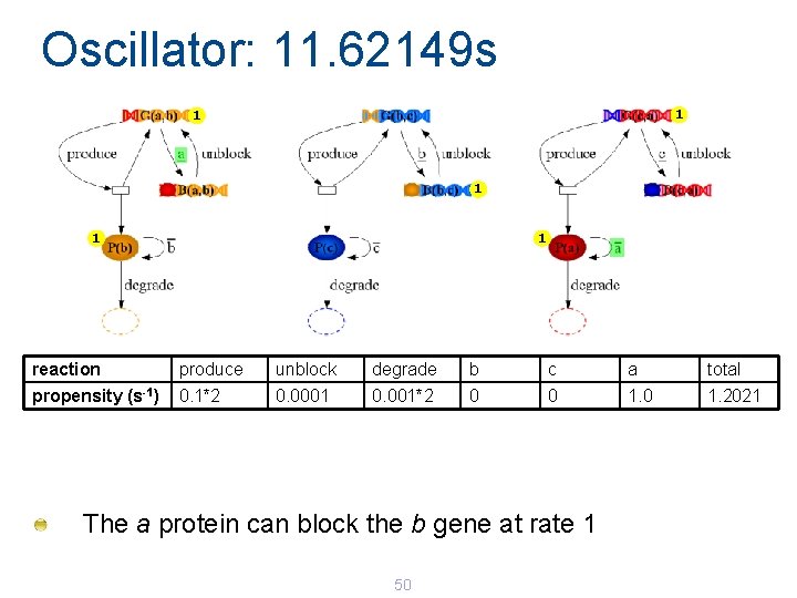
Oscillator: 11. 62149 s 1 1 1 reaction produce unblock degrade b c a total propensity (s-1) 0. 1*2 0. 0001 0. 001*2 0 0 1. 2021 The a protein can block the b gene at rate 1 50
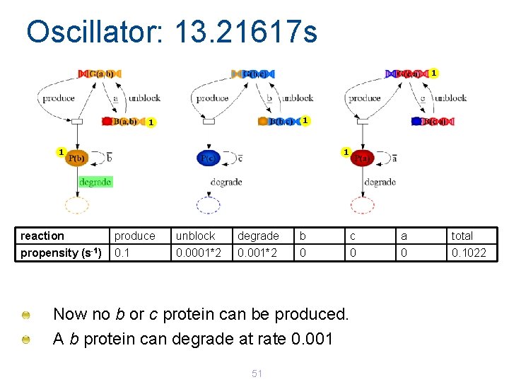
Oscillator: 13. 21617 s 1 1 1 reaction produce unblock degrade b c a total propensity (s-1) 0. 1 0. 0001*2 0 0. 1022 Now no b or c protein can be produced. A b protein can degrade at rate 0. 001 51
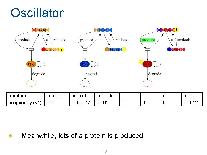
Oscillator 1 1 reaction produce unblock degrade b c a total propensity (s-1) 0. 1 0. 0001*2 0. 001 0 0. 1012 Meanwhile, lots of a protein is produced 52
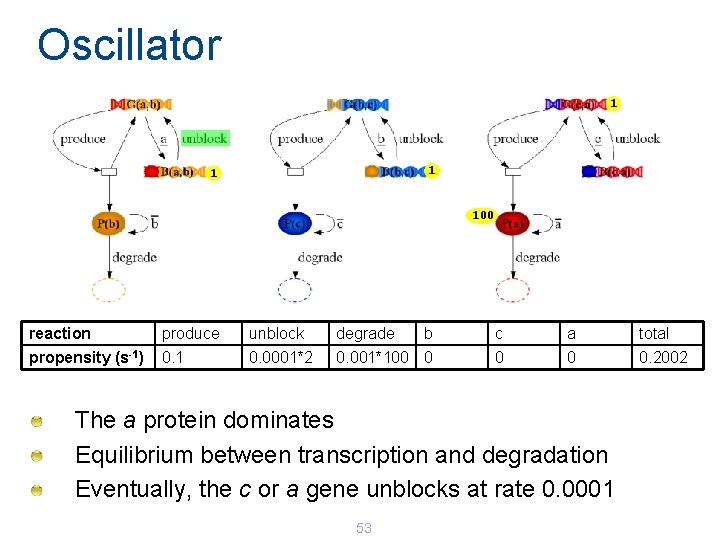
Oscillator 1 100 reaction produce unblock degrade b c a total propensity (s-1) 0. 1 0. 0001*2 0. 001*100 0 0. 2002 The a protein dominates Equilibrium between transcription and degradation Eventually, the c or a gene unblocks at rate 0. 0001 53
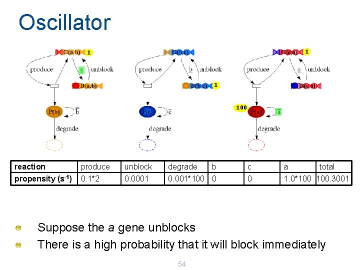
Oscillator 1 100 reaction produce unblock degrade b c a total propensity (s-1) 0. 1*2 0. 0001 0. 001*100 0 0 1. 0*100 100. 3001 Suppose the a gene unblocks There is a high probability that it will block immediately 54
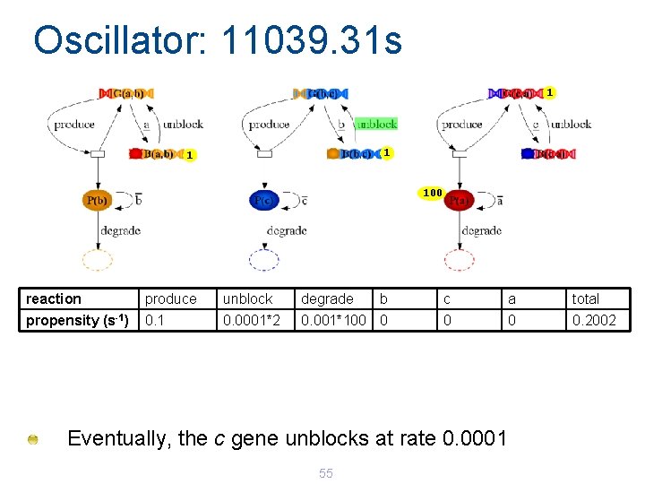
Oscillator: 11039. 31 s 1 100 reaction produce unblock degrade b c a total propensity (s-1) 0. 1 0. 0001*2 0. 001*100 0 0. 2002 Eventually, the c gene unblocks at rate 0. 0001 55
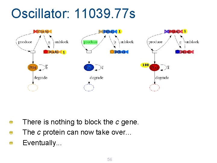
Oscillator: 11039. 77 s 1 100 There is nothing to block the c gene. The c protein can now take over. . . Eventually. . . 56
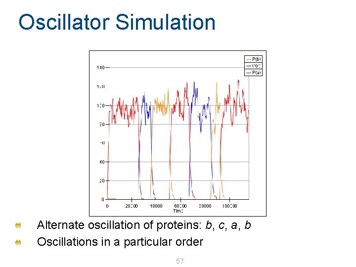
Oscillator Simulation Alternate oscillation of proteins: b, c, a, b Oscillations in a particular order 57
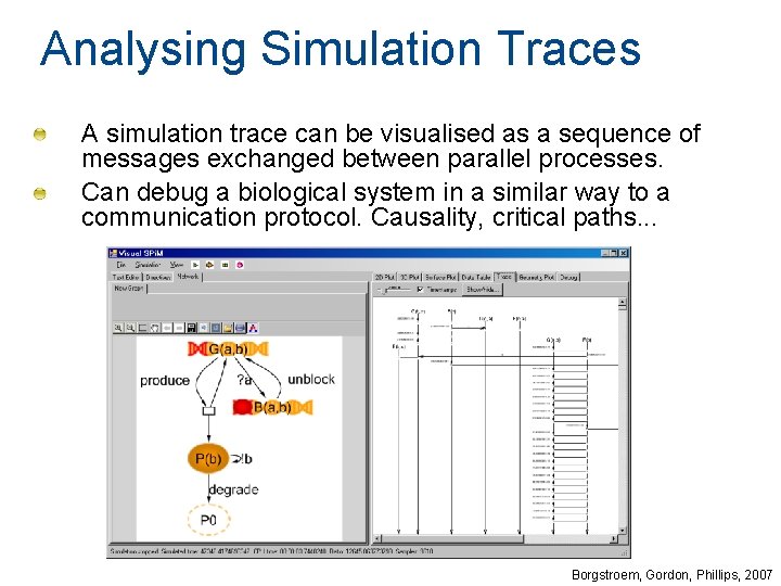
Analysing Simulation Traces A simulation trace can be visualised as a sequence of messages exchanged between parallel processes. Can debug a biological system in a similar way to a communication protocol. Causality, critical paths. . . Borgstroem, Gordon, Phillips, 2007
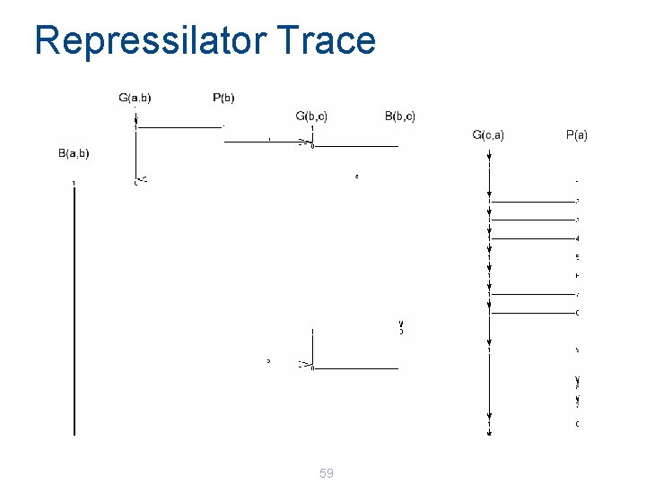
Repressilator Trace 59
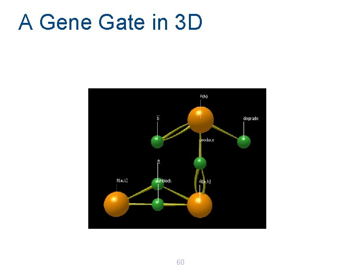
A Gene Gate in 3 D 60
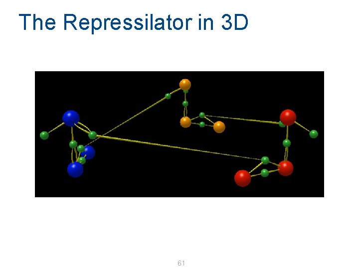
The Repressilator in 3 D 61
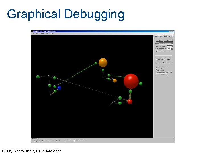
Graphical Debugging GUI by Rich Williams, MSR Cambridge
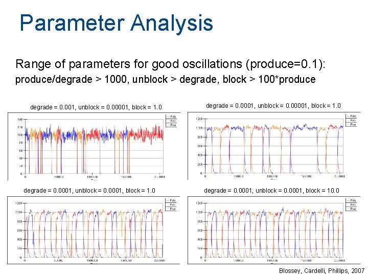
Parameter Analysis Range of parameters for good oscillations (produce=0. 1): produce/degrade > 1000, unblock > degrade, block > 100*produce degrade = 0. 001, unblock = 0. 00001, block = 1. 0 degrade = 0. 0001, unblock = 0. 0001, block = 10. 0 Blossey, Cardelli, Phillips, 2007
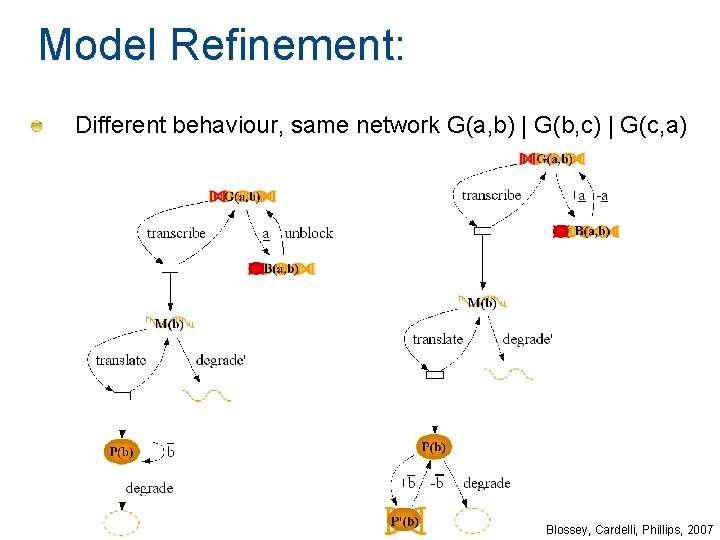
Model Refinement: Different behaviour, same network G(a, b) | G(b, c) | G(c, a) Blossey, Cardelli, Phillips, 2007
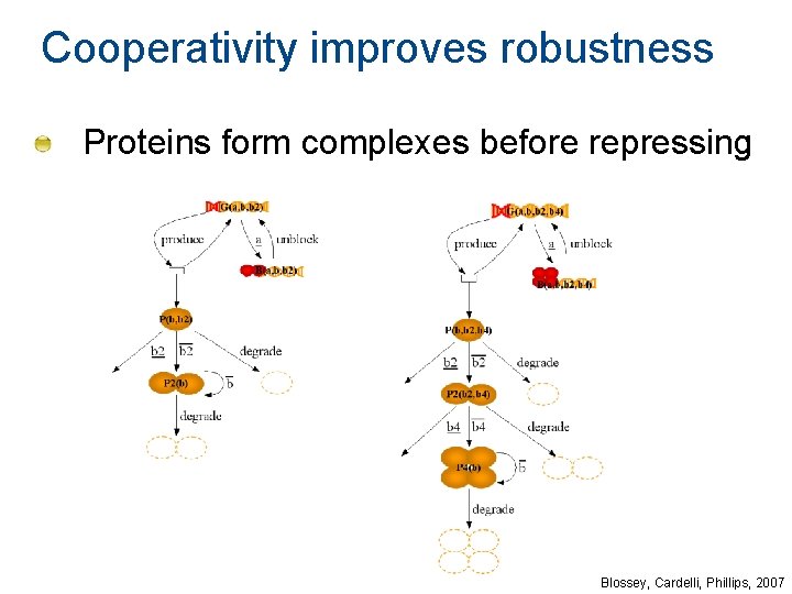
Cooperativity improves robustness Proteins form complexes before repressing Blossey, Cardelli, Phillips, 2007
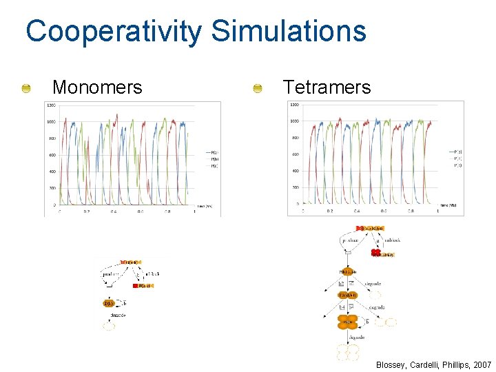
Cooperativity Simulations Monomers Tetramers Blossey, Cardelli, Phillips, 2007
![Bacteria Logic Gates [Guet et al. , 2002] © 2002 AAAS. Reprinted with permission Bacteria Logic Gates [Guet et al. , 2002] © 2002 AAAS. Reprinted with permission](http://slidetodoc.com/presentation_image_h2/53d5aaf19256564706e65910e40b97de/image-67.jpg)
Bacteria Logic Gates [Guet et al. , 2002] © 2002 AAAS. Reprinted with permission from Guet et al. Combinatorial Synthesis of Genetic Networks. Science 296 (5572): 1466 - 1470 3 genes: tet. R, lac. I, lc. I 5 promoters: PL 1, PL 2, PT, Pl-, Pl+ 125 possible networks consisting of 3 promoter-gene units 2 inputs: IPTG (represses Lac), a. Tc (represses Tet) 1 output: GFP (linked to Pl-) Blossey, Cardelli, Phillips, 2006
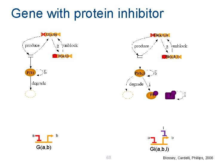
Gene with protein inhibitor G(a, b) Gi(a, b, i) 68 Blossey, Cardelli, Phillips, 2006
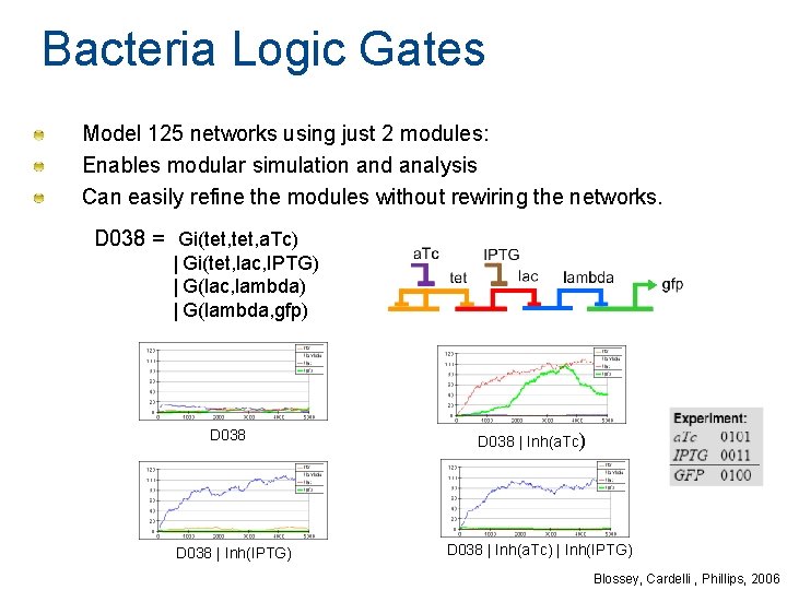
Bacteria Logic Gates Model 125 networks using just 2 modules: Enables modular simulation and analysis Can easily refine the modules without rewiring the networks. D 038 = Gi(tet, a. Tc) | Gi(tet, lac, IPTG) | G(lac, lambda) | G(lambda, gfp) D 038 | Inh(IPTG) D 038 | Inh(a. Tc) | Inh(IPTG) Blossey, Cardelli , Phillips, 2006

A Computational Model of C. elegans Vulval Development with Rosie Bloxsom (Cambridge University) Tim Labeeuw (Cambridge University) Jasmin Fisher (MSR Cambridge) Hillel Kugler (MSR Cambridge)
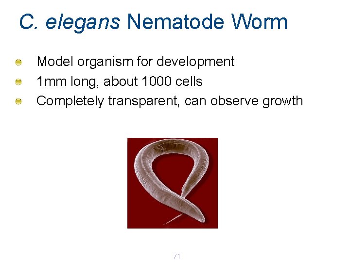
C. elegans Nematode Worm Model organism for development 1 mm long, about 1000 cells Completely transparent, can observe growth 71
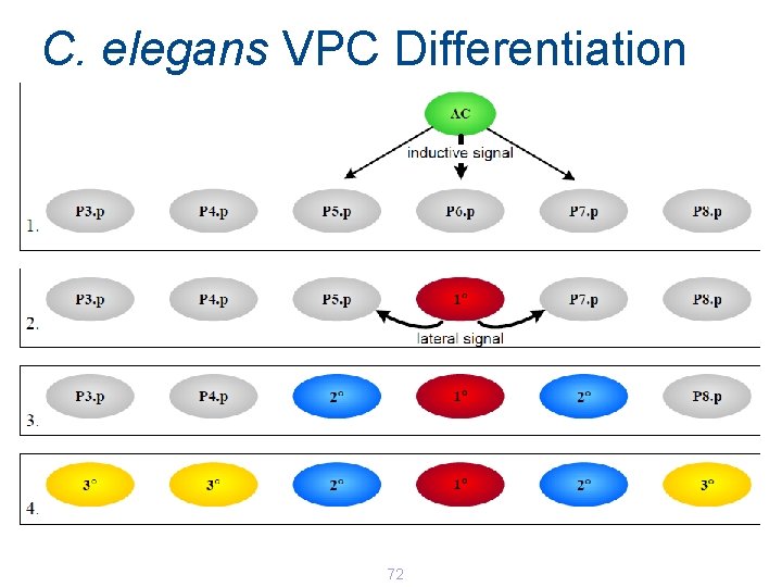
C. elegans VPC Differentiation 72
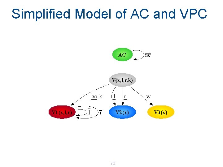
Simplified Model of AC and VPC 73
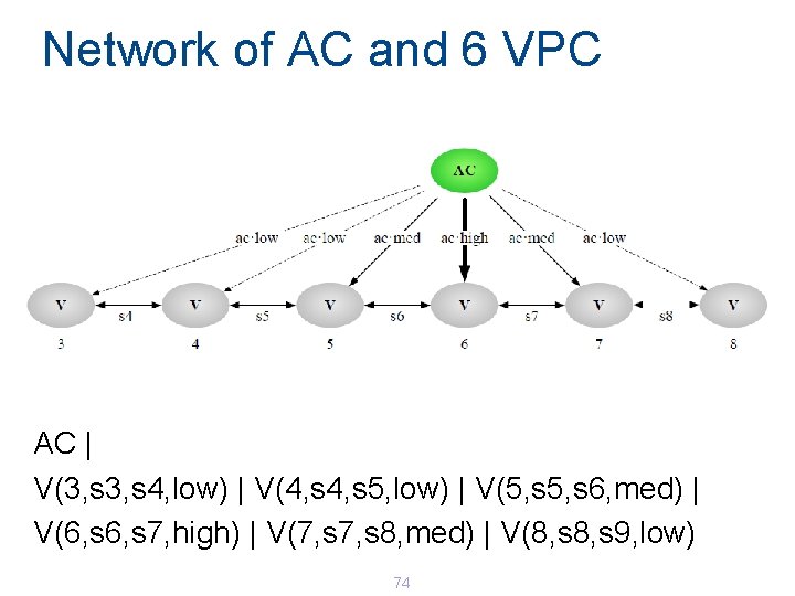
Network of AC and 6 VPC AC | V(3, s 4, low) | V(4, s 5, low) | V(5, s 6, med) | V(6, s 7, high) | V(7, s 8, med) | V(8, s 9, low) 74
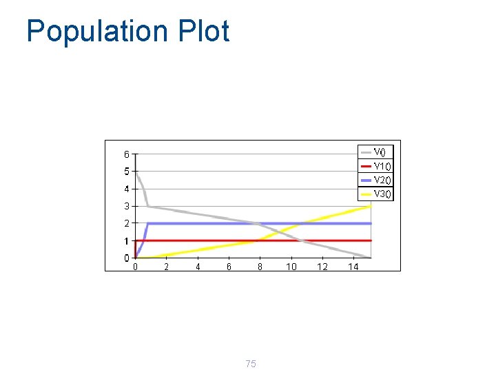
Population Plot 75
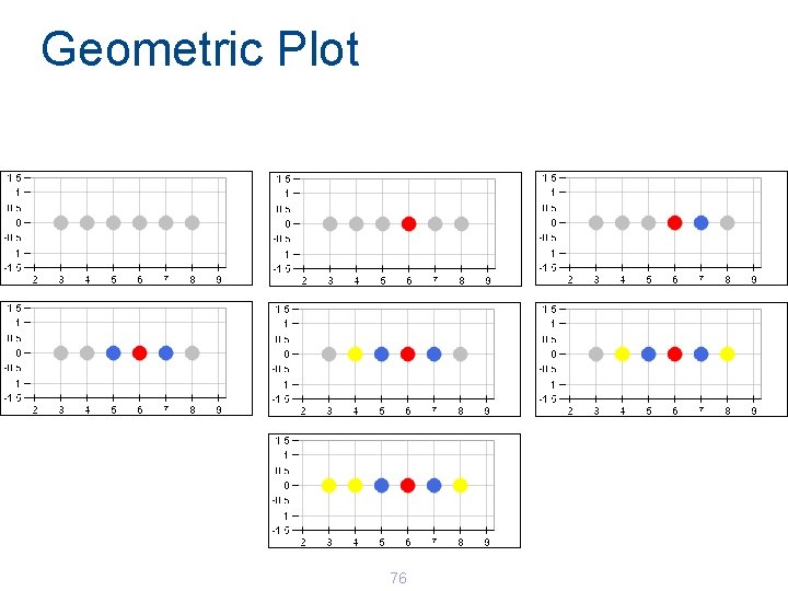
Geometric Plot 76
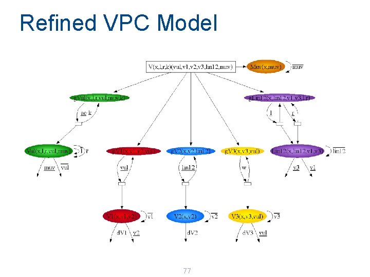
Refined VPC Model 77
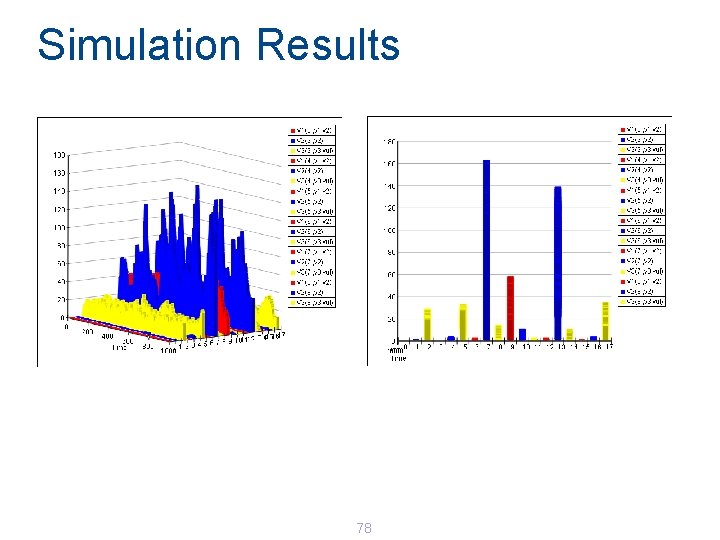
Simulation Results 78

A Computational Model of MHC class I Antigen Presentation with Luca Cardelli (MSR Cambridge) Leonard Goldstein (Cambridge University) Tim Elliott (Southampton University) Joern Werner (Southampton University)

MHC: A Biological Virus Scanner © 2005 from Immunobiology, Sixth Edition by Janeway et al. Reproduced by permission of Garland Science/Taylor & Francis LLC. 80

MHC: A Biological Virus Scanner © 2005 from Immunobiology, Sixth Edition by Janeway et al. Reproduced by permission of Garland Science/Taylor & Francis LLC. 81
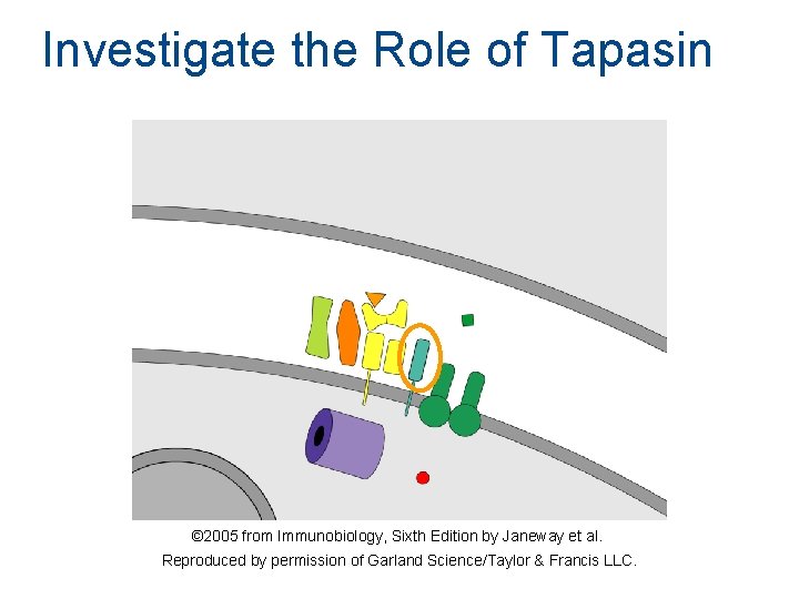
Investigate the Role of Tapasin © 2005 from Immunobiology, Sixth Edition by Janeway et al. Reproduced by permission of Garland Science/Taylor & Francis LLC.
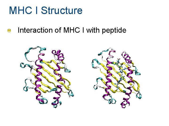
MHC I Structure Interaction of MHC I with peptide
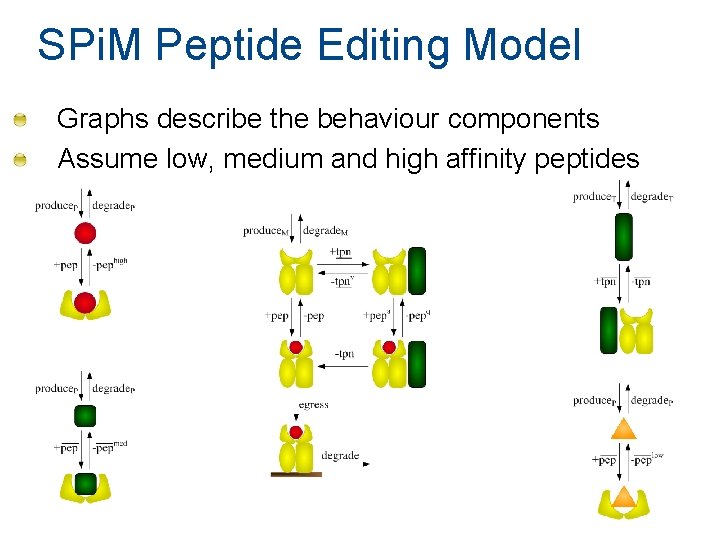
SPi. M Peptide Editing Model Graphs describe the behaviour components Assume low, medium and high affinity peptides
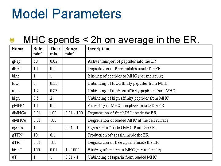
Model Parameters MHC spends < 2 h on average in the ER. Name Rate min-1 Time min Range min-1 g. Pep 50 0. 02 Active transport of peptides into the ER d. Pep 10 0. 1 Degradation of free peptides inside the ER bind 1 1 Binding of peptides to MHC (per molecule) low 3 0. 33 Unbinding of low affinity peptides from MHC med 1. 2 0. 83 Unbinding of medium affinity peptides from MHC high 0. 5 2 Unbinding of high affinity peptides from MHC g. MHC 10 0. 1 Assembly of MHC complexes inside the ER d. MHCo 0. 01 100 d. MHCe 0. 01 100 egress 1 1 g. TPN 10 0. 1 Production of tapasin inside the ER d. TPN 0. 01 100 Degradation of free tapasin inside the ER bind. T 100 0. 01 1 - 1000 Binding of tapasin to MHC (per molecule) u. T 1 1 0. 01 - 1 Unbinding of tapasin from loaded MHC 0. 01 - 100 Description Degradation of free MHC inside the ER Degradation of loaded MHC at the cell surface 0. 01 - 1 Egression of loaded MHC from the ER
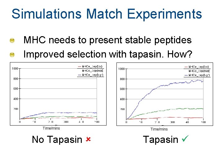
Simulations Match Experiments MHC needs to present stable peptides Improved selection with tapasin. How? Time/mins No Tapasin Time/mins Tapasin
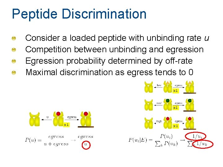
Peptide Discrimination Consider a loaded peptide with unbinding rate u Competition between unbinding and egression Egression probability determined by off-rate Maximal discrimination as egress tends to 0 x 1 x 1
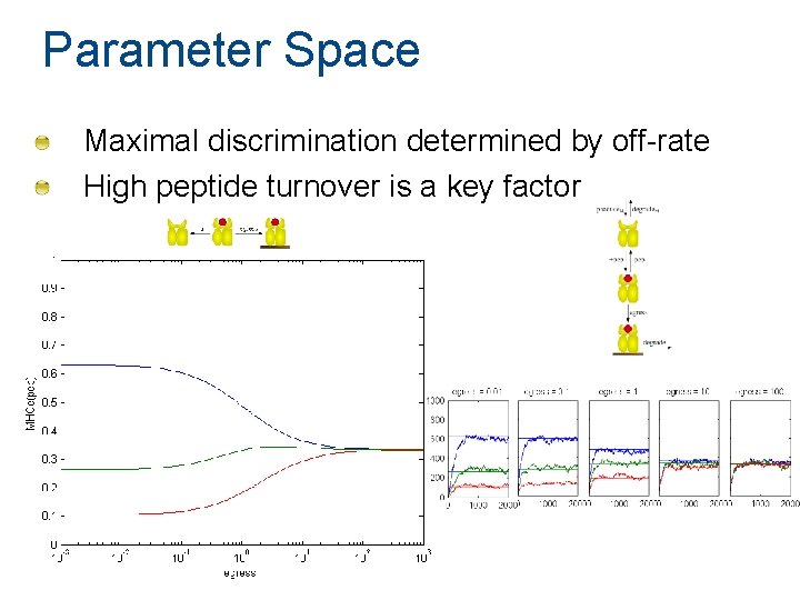
Parameter Space Maximal discrimination determined by off-rate High peptide turnover is a key factor
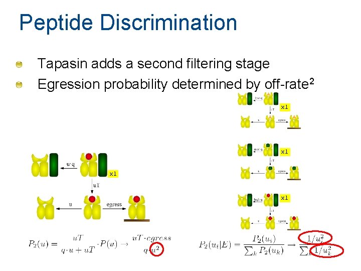
Peptide Discrimination Tapasin adds a second filtering stage Egression probability determined by off-rate 2 x 1 x 1
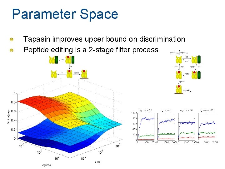
Parameter Space Tapasin improves upper bound on discrimination Peptide editing is a 2 -stage filter process
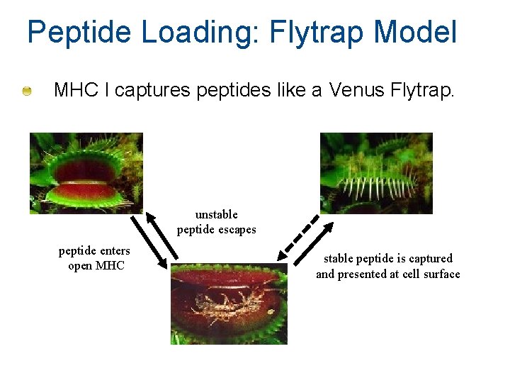
Peptide Loading: Flytrap Model MHC I captures peptides like a Venus Flytrap. unstable peptide escapes peptide enters open MHC stable peptide is captured and presented at cell surface
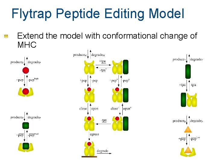
Flytrap Peptide Editing Model Extend the model with conformational change of MHC
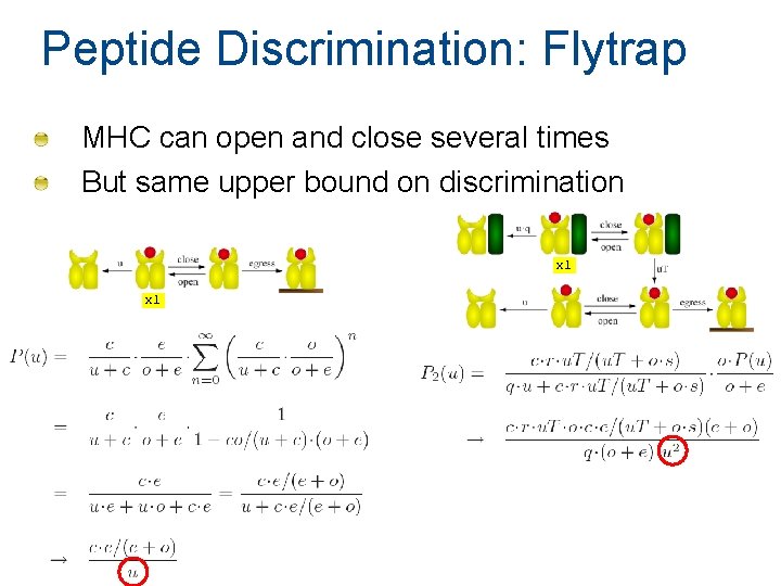
Peptide Discrimination: Flytrap MHC can open and close several times But same upper bound on discrimination x 1
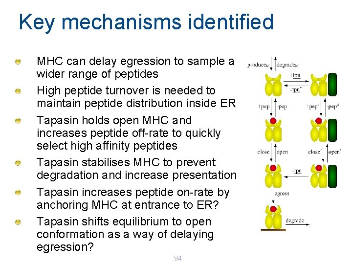
Key mechanisms identified MHC can delay egression to sample a wider range of peptides High peptide turnover is needed to maintain peptide distribution inside ER Tapasin holds open MHC and increases peptide off-rate to quickly select high affinity peptides Tapasin stabilises MHC to prevent degradation and increase presentation Tapasin increases peptide on-rate by anchoring MHC at entrance to ER? Tapasin shifts equilibrium to open conformation as a way of delaying egression? 94
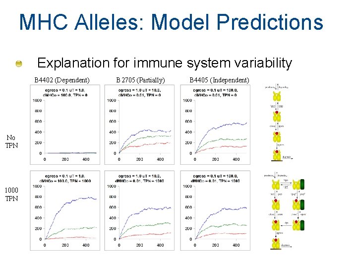
MHC Alleles: Model Predictions Explanation for immune system variability B 4402 (Dependent) No TPN 1000 TPN B 2705 (Partially) B 4405 (Independent)
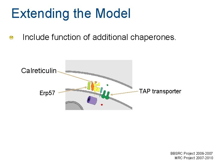
Extending the Model Include function of additional chaperones. Calreticulin Erp 57 TAP transporter BBSRC Project 2006 -2007 MRC Project 2007 -2010
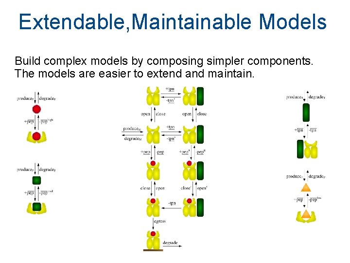
Extendable, Maintainable Models Build complex models by composing simpler components. The models are easier to extend and maintain.
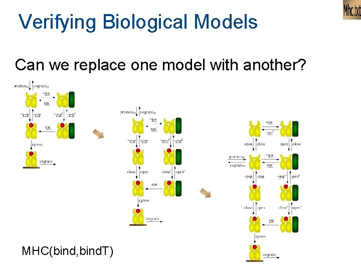
Verifying Biological Models Can we replace one model with another? MHC(bind, bind. T)
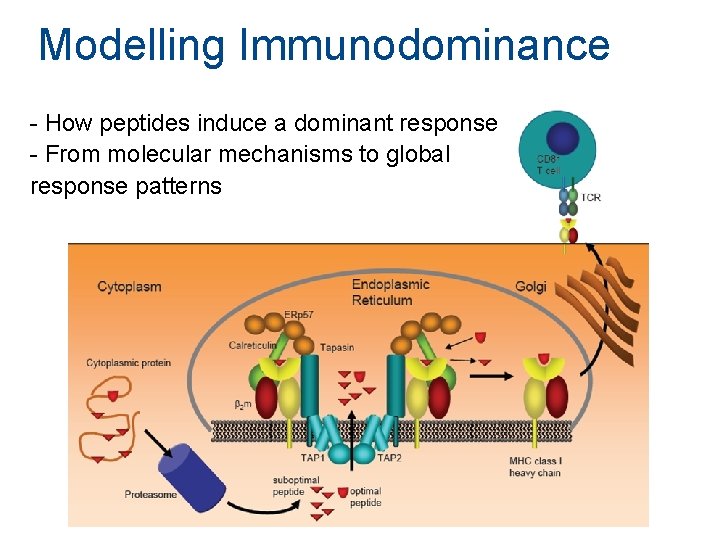
Modelling Immunodominance - How peptides induce a dominant response - From molecular mechanisms to global response patterns
![References [Blossey et al. , 2007] Blossey, R. , Cardelli, L. , and Phillips, References [Blossey et al. , 2007] Blossey, R. , Cardelli, L. , and Phillips,](http://slidetodoc.com/presentation_image_h2/53d5aaf19256564706e65910e40b97de/image-100.jpg)
References [Blossey et al. , 2007] Blossey, R. , Cardelli, L. , and Phillips, A. (2007). Compositionality, Stochasticity and Cooperativity in Dynamic Models of Gene Regulation. HFSP Journal. [Blossey et al. , 2006] Blossey, R. , Cardelli, L. , and Phillips, A. (2006). A compositional approach to the stochastic dynamics of gene networks. Transactions in Computational Systems Biology, 3939: 99– 122. [Borgstroem et al. , 2007] Borgstroem, J. Gordon, A. , and Phillips, A. (2007). A Chart Semantics for the Pi-calculus. In Proceedings of Expressiveness in Concurrency. [Gillespie, 1977] Gillespie, D. T. (1977). Exact stochastic simulation of coupled chemical reactions. J. Phys. Chem. , 81(25): 2340– 2361. [Guet et al. , 2002] Guet, C. C. , Elowitz, M. B. , Hsing, W. & Leibler, S. (2002) Combinatorial synthesis of genetic networks. Science 296 1466 -1470. [Huang and Ferrel, 1996] Huang, C. -Y. F. and Ferrel, J. E. (1996). Ultrasensitivity of the mitogenactivated protein kinase cascade. PNAS, 93: 10078– 10083. [Lecca and Priami, 2003] Lecca, P. and Priami, C. (2003). Cell cycle control in eukaryotes: a biospi model. In proceedings of Concurrent Models in Molecular Biology. [Phillips and Cardelli, 2007] Phillips, A. and Cardelli, L. (2007). Efficient, Correct Simulation of Biological Processes in the Stochastic Pi-calculus. In Proceedings of Computational Methods in Systems Biology, 4695: 184– 199. [Phillips et al. , 2006] Phillips, A. , Cardelli, L. , and Castagna, G. (2006). A graphical representation for biological processes in the stochastic pi-calculus. Transactions in Computational Systems Biology, 4230: 123– 152.
![References [Priami, 1995] Priami, C. (1995). Stochastic p-calculus. The Computer Journal, 38(6): 578– 589. References [Priami, 1995] Priami, C. (1995). Stochastic p-calculus. The Computer Journal, 38(6): 578– 589.](http://slidetodoc.com/presentation_image_h2/53d5aaf19256564706e65910e40b97de/image-101.jpg)
References [Priami, 1995] Priami, C. (1995). Stochastic p-calculus. The Computer Journal, 38(6): 578– 589. Proceedings of PAPM’ 95. [Priami et al. , 2001] Priami, C. , Regev, A. , Shapiro, E. , and Silverman, W. (2001). Application of a stochastic name-passing calculus to representation and simulation of molecular processes. Information Processing Letters, 80: 25– 31. [Regev et al. , 2001] Regev, A. , Silverman, W. , and Shapiro, E. (2001). Representation and simulation of biochemical processes using the pi- calculus process algebra. In Altman, R. B. , Dunker, A. K. , Hunter, L. , and Klein, T. E. , editors, Pacific Symposium on Biocomputing, volume 6, pages 459– 470, Singapore. World Scientific Press. [Sangiorgi and Walker, 2001] Sangiorgi, D. and Walker, D. (2001). The pi-calculus: a Theory of Mobile Processes. Cambridge University Press. [Silverman et al. , 1987] Silverman, W. , Hirsch, M. , Houri, A. , and Shapiro, E. (1987). The logix system user manual, version 1. 21. In Shapiro, E. , editor, Concurrent Prolog: Collected Papers (Volume II), pages 46– 77. MIT Press, London. Mark Howarth, Anthony Williams, Anne B. Tolstrup, and Tim Elliott. Tapasin enhances mhc class i peptide presentation according to peptide half-life. PNAS, 101(32): 11737– 11742, 2004. Sebastian Springer, Klaus Doring, Jonathan C. A. Skipper, Alain R. M. Townsend, and Vincenzo Cerundolo. Fast association rates suggest a conformational change in the mhc class i molecule h 2 db upon peptide binding. Biochemistry, 37: 3001– 3012, 1998. A. Williams, C. Au Peh, and T. Elliott. The cell biology of mhc class i antigen presentation. Tissue Antigens, 59: 3– 17, 2002.
SPi. M Definition Syntax Semantics Graphics
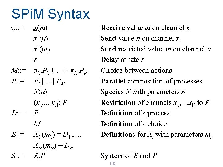
SPi. M Syntax p: : = M: : = P: : = D: : = E: : = S: : = x(m) _ x n _ x (m) r p 1. P 1 +. . . + p. N. PN P 1 |. . . | PM X(n) (x 1, . . . , x. N) P P M X 1 (m 1) = D 1 , . . . , XN (m. N) = DN E, P Receive value m on channel x Send value n on channel x Send restricted value m on channel x Delay at rate r Choice between actions Parallel composition of processes Species X with parameters n Restriction of channels x 1, . . . , x. N to P Definition of a process Definition of a choice Definitions for Xi with parameters mi System of E and P 103
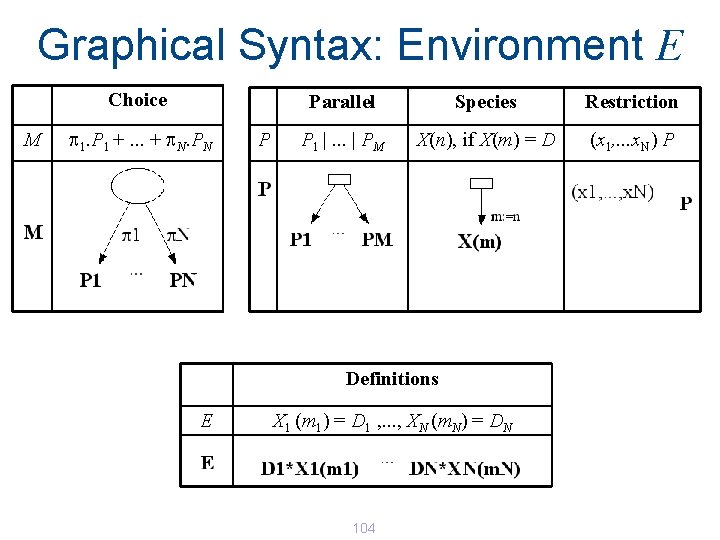
Graphical Syntax: Environment E Choice M p 1. P 1 +. . . + p. N. PN P Parallel Species Restriction P 1 |. . . | PM X(n), if X(m) = D (x 1, . . . x. N) P Definitions E X 1 (m 1) = D 1 , . . . , XN (m. N) = DN 104
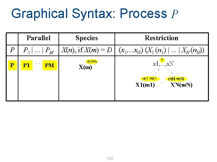
Graphical Syntax: Process P Parallel P P 1 |. . . | PM Species Restriction X(n), if X(m) = D (x 1, . . . x. N) (X 1 (n 1) |. . . | XN (n. N)) 105
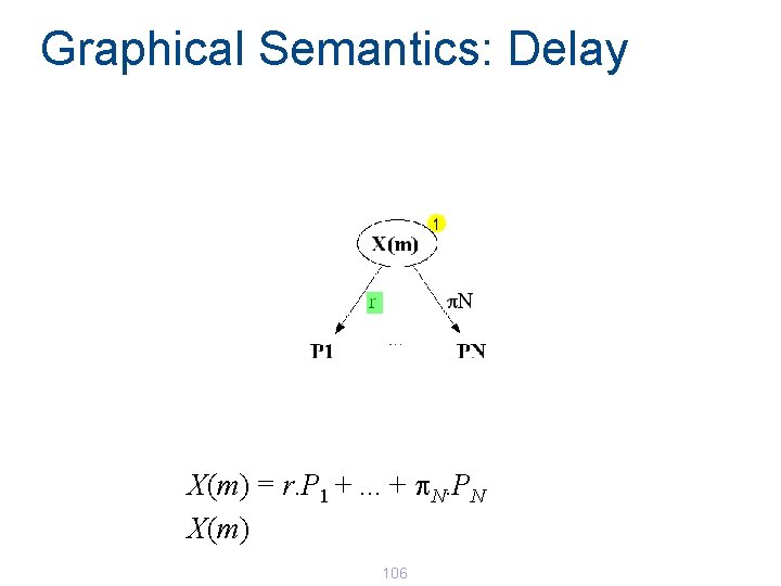
Graphical Semantics: Delay X(m) = r. P 1 +. . . + p. N. PN X(m) 106
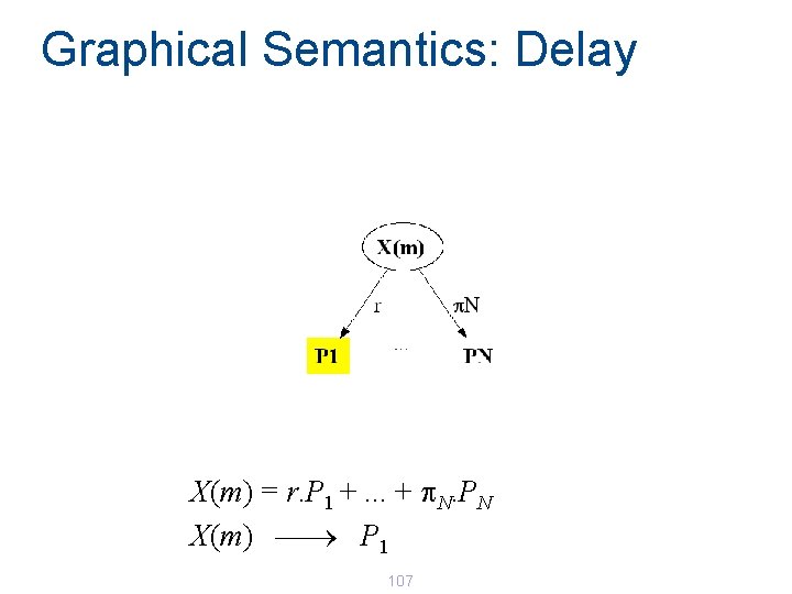
Graphical Semantics: Delay X(m) = r. P 1 +. . . + p. N. PN X(m) ¾ P 1 107
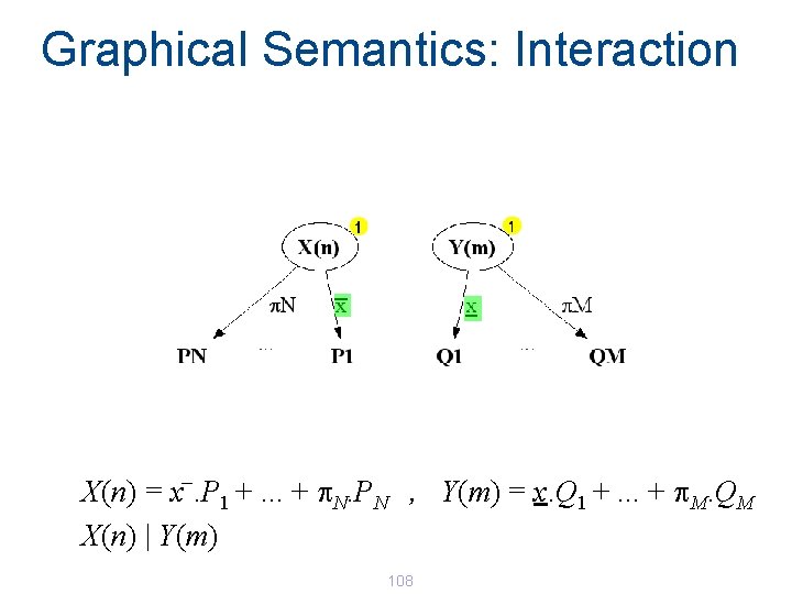
Graphical Semantics: Interaction _ X(n) = x. P 1 +. . . + p. N. PN , Y(m) = x. Q 1 +. . . + p. M. QM X(n) | Y(m) 108
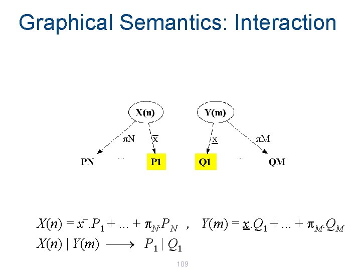
Graphical Semantics: Interaction _ X(n) = x. P 1 +. . . + p. N. PN , Y(m) = x. Q 1 +. . . + p. M. QM X(n) | Y(m) ¾ P 1 | Q 1 109
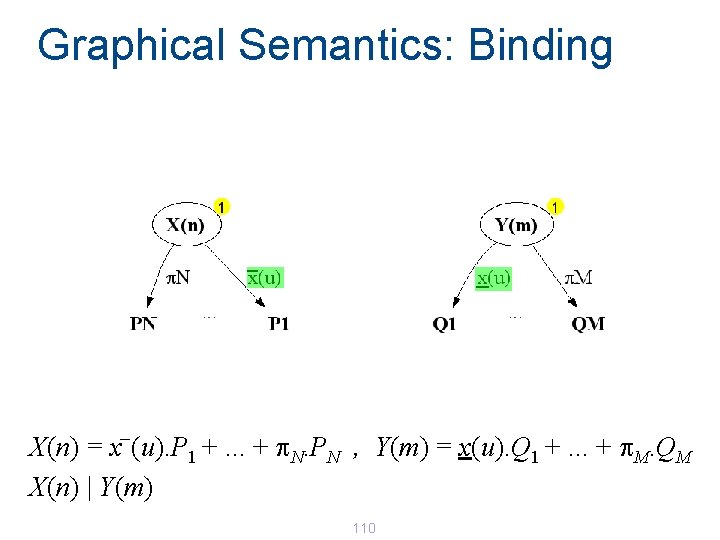
Graphical Semantics: Binding _ X(n) = x (u). P 1 +. . . + p. N. PN , Y(m) = x(u). Q 1 +. . . + p. M. QM X(n) | Y(m) 110
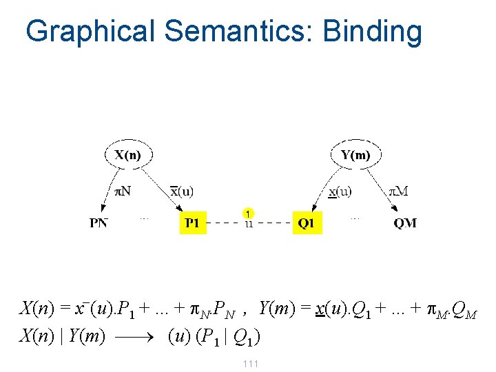
Graphical Semantics: Binding _ X(n) = x (u). P 1 +. . . + p. N. PN , Y(m) = x(u). Q 1 +. . . + p. M. QM X(n) | Y(m) ¾ (u) (P 1 | Q 1) 111
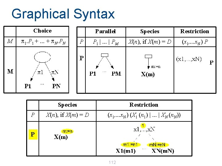
Graphical Syntax Choice M p 1. P 1 +. . . + p. N. PN P P Parallel Species Restriction P 1 |. . . | PM X(n), if X(m) = D (x 1, . . . x. N) P Species Restriction X(n), if X(m) = D (x 1, . . . x. N) (X 1 (n 1) |. . . | XN (n. N)) 112
- Slides: 112