A VIEW OF THE EM ALGORITHM THAT JUSTIFIES

A VIEW OF THE EM ALGORITHM THAT JUSTIFIES INCREMENTAL, SPARSE, AND OTHER VARIANTS RADFORD M. NEAL GEOFFREY E. HINTON 발표: 황규백

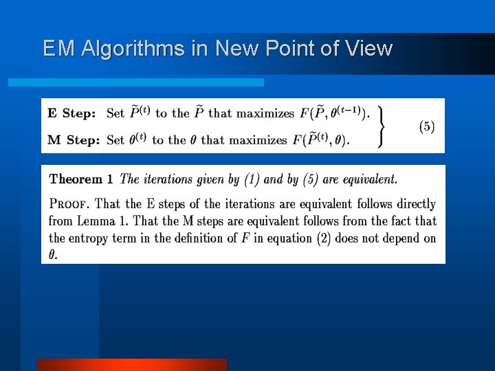
Abstract l First, the concept of “the negative free energy” is introduced. 4 E step maximizes this with respect to the distribution over unobserved variables. 4 M step also maximizes this with respect to the model parameters. l Then, it is easy to justify an incremental variant of the EM algorithm. 4 Also, for sparse algorithm, and other variants

Introduction l EM algorithms find maximum likelihood parameter estimates in problems where some variables were unobserved. 4 It can be shown that each iteration improves the true likelihood, or leaves it unchanged. l The M step can be partially implemented. 4 Not maximizing, but improving 4 Generalized EM algorithm, ECM l The E step can also be partially implemented. 4 Incremental EM algorithm • The unobserved variables are commonly independent.

Introduction(cont’d) l A view of the EM algorithm here 4 Maximizing the joint function of the parameters and of the distribution over the unobserved variables. 4 And this is analogous to the “free energy” function used in statistical physics. 4 This can also be viewed as Kullback-Leibler divergence. 4 E step maximizes this function with respect to the distribution over unobserved variables. 4 M step also maximizes this function with respect to the model parameters.

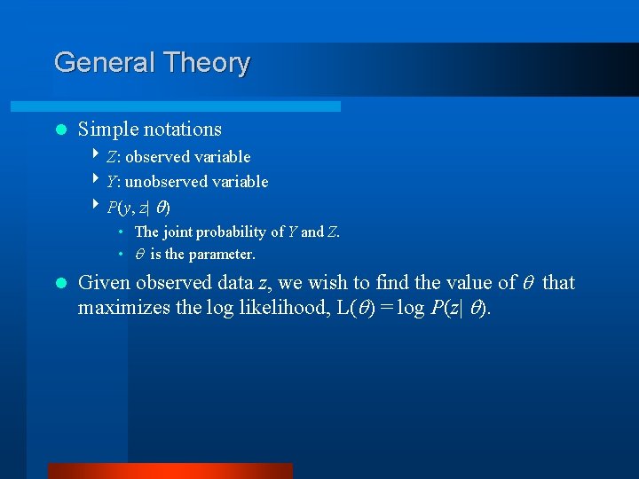
General Theory l Simple notations 4 Z: observed variable 4 Y: unobserved variable 4 P(y, z| ) • The joint probability of Y and Z. • is the parameter. l Given observed data z, we wish to find the value of that maximizes the log likelihood, L( ) = log P(z| ).

EM Algorithm l EM algorithms start with initial guess at the parameter (0) and then proceeds following steps. 4 Each iteration improves, or leaves unchanged the true likelihood. 4 The algorithm converges to a local maximum of L( ). l GEM algorithm is also guaranteed to converge.

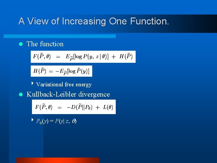
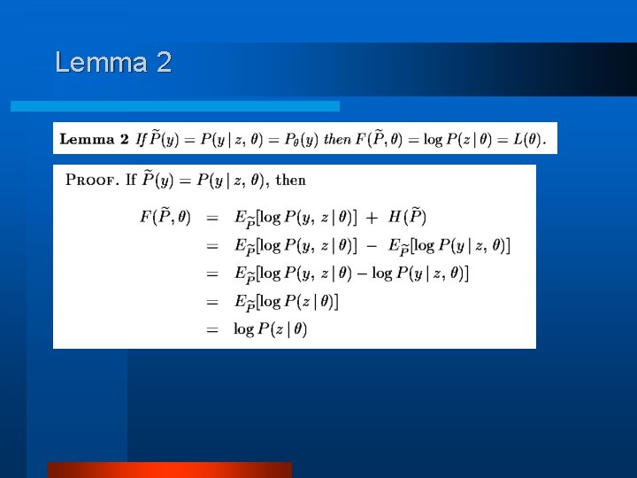
A View of Increasing One Function. l The function 4 Variational free energy l Kullback-Leibler divergence 4 P (y) = P(y| z, )

Lemma 1

Lemma 2

EM Algorithms in New Point of View

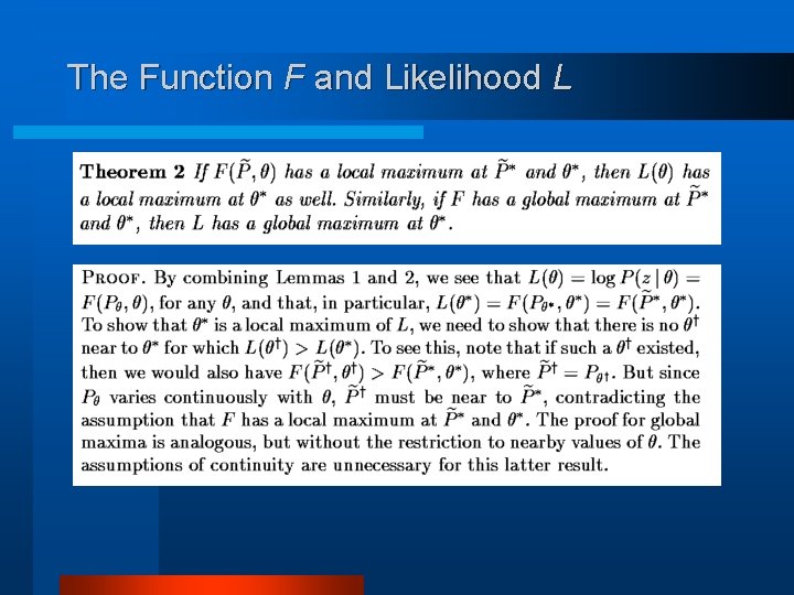
The Function F and Likelihood L

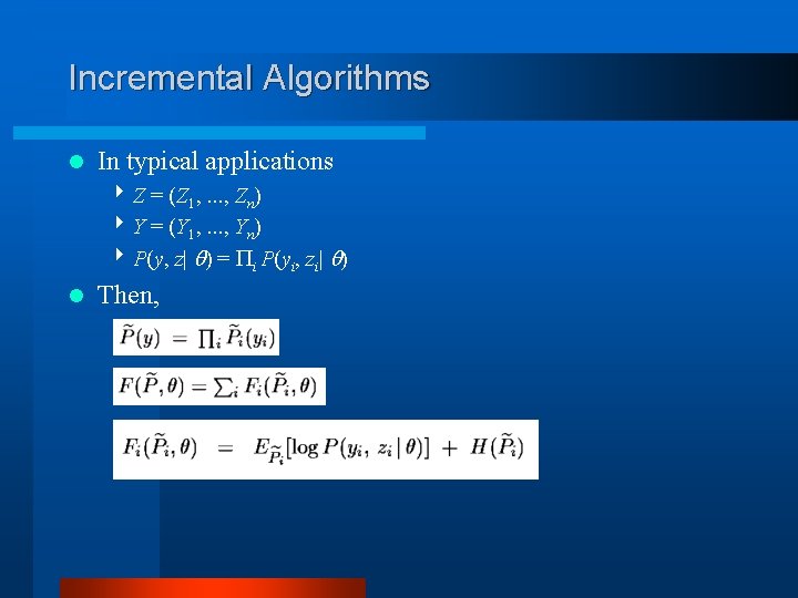
Incremental Algorithms l In typical applications 4 Z = (Z 1, . . . , Zn) 4 Y = (Y 1, . . . , Yn) 4 P(y, z| ) = i P(yi, zi| ) l Then,

Incremental Algorithms(cont’d) l So, the algorithm is

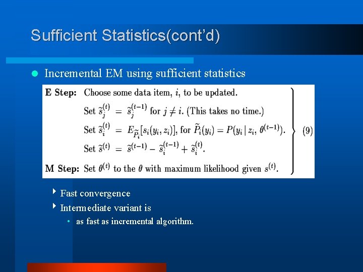
Sufficient Statistics l Vector of sufficient statistics 4 s(y, z) = i si(yi, zi) l Standard EM Algorithm using sufficient statistics

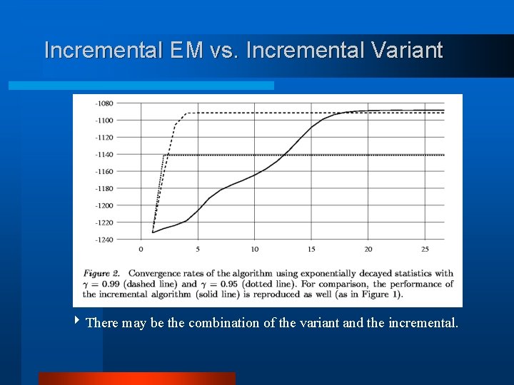
Sufficient Statistics(cont’d) l Incremental EM using sufficient statistics 4 Fast convergence 4 Intermediate variant is • as fast as incremental algorithm.

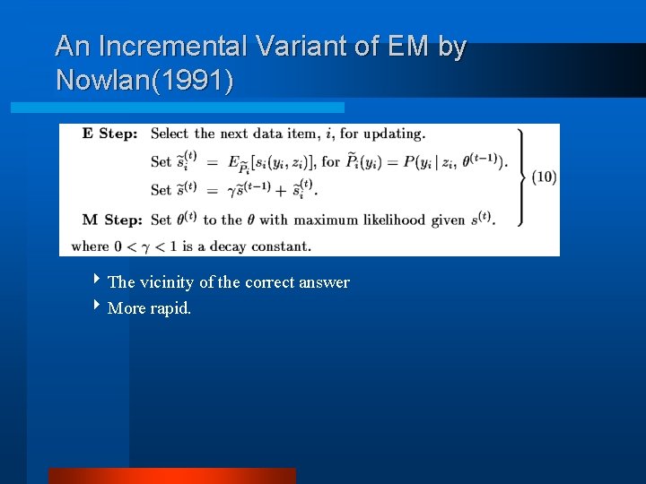
An Incremental Variant of EM by Nowlan(1991) 4 The vicinity of the correct answer 4 More rapid.

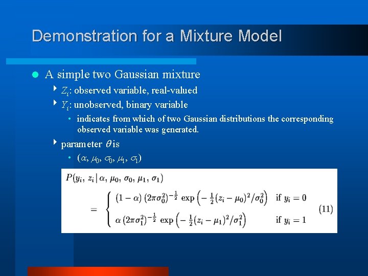
Demonstration for a Mixture Model l A simple two Gaussian mixture 4 Zi: observed variable, real-valued 4 Yi: unobserved, binary variable • indicates from which of two Gaussian distributions the corresponding observed variable was generated. 4 parameter is • ( , 0 , 1 )

Gaussian Mixture Model l Sufficient statistics

Standard EM vs. Incremental EM 4 But, the computation time in a pass of incremental EM is as twice as that of standard EM.

Incremental EM vs. Incremental Variant 4 There may be the combination of the variant and the incremental.

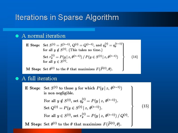
A Sparse Algorithm l A “sparse” variant of the EM algorithm may be advantageous 4 when the unobserved variable, Y, can take on many possible values, but only a small set of “plausible” values have nonnegligible probability. l Update only “plausible” values. 4 At infrequent intervals, all probabilities are recomputed, and the “plausible” set is changed. l In detail,

Iterations in Sparse Algorithm l A normal iteration l A full iteration

Other Variants l “Winner-take-all” variant of EM algorithm 4 Early stages of maximizing F 4 In estimating Hidden Markov Models for speech recognition