A Speaker Pruning Algorithm for RealTime Speaker Identification
- Slides: 16

A Speaker Pruning Algorithm for Real-Time Speaker Identification Tomi Kinnunen, Evgeny Karpov, Pasi Fränti University of Joensuu, FINLAND Department of Computer Science AVBPA 2003 Guildford, UK, June 9 -11, 2003

Abstract • Speaker identification task is computationally very expensive • Most computation originates from calculating the matching scores • Proposed method: drop out unlikely speakers “on the fly” • Reduced computation time with slightly increased error rate

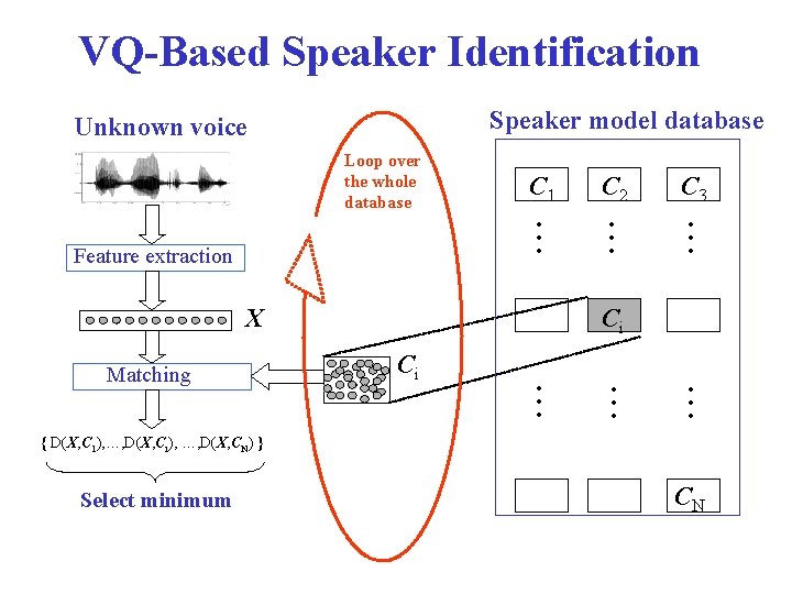
VQ-Based Speaker Identification Speaker model database Unknown voice Loop over the whole database C 1 C 2 C 3 . . Feature extraction X Ci . . Matching Ci { D(X, C 1), …, D(X, Ci), …, D(X, CN) } Select minimum CN

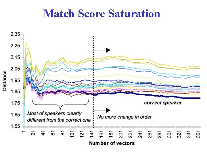
Match Score Saturation

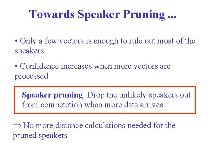
Towards Speaker Pruning. . . • Only a few vectors is enough to rule out most of the speakers • Confidence increases when more vectors are processed Speaker pruning: Drop the unlikely speakers out from competetion when more data arrives No more distance calculations needed for the pruned speakers

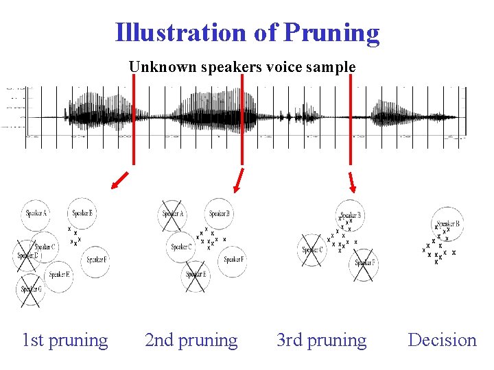
Illustration of Pruning Unknown speakers voice sample 1 st pruning 2 nd pruning 3 rd pruning Decision

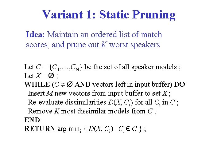
Variant 1: Static Pruning Idea: Maintain an ordered list of match scores, and prune out K worst speakers Let C = {C 1, …, CN} be the set of all speaker models ; Let X = Ø ; WHILE (C ≠ Ø AND vectors left in input buffer) DO Insert M new vectors from input buffer to set X ; Re-evaluate dissimilarities D(X, Ci) for all Ci in C ; Remove K most dissimilar models from C ; END RETURN arg mini { D(X, Ci) | Ci Є C } ;

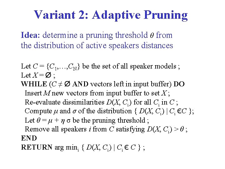
Variant 2: Adaptive Pruning Idea: determine a pruning threshold θ from the distribution of active speakers distances Let C = {C 1, …, CN} be the set of all speaker models ; Let X = Ø ; WHILE (C ≠ Ø AND vectors left in input buffer) DO Insert M new vectors from input buffer to set X ; Re-evaluate dissimilarities D(X, Ci) for all Ci in C ; Compute μ and σ of the distribution { D(X, Ci) | Ci ЄC }; Let θ = μ + η σ be the pruning threshold ; Remove all speakers i from C satisfying D(X, Ci) > θ ; END RETURN arg mini { D(X, Ci) | Ci Є C } ;

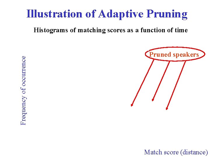
Illustration of Adaptive Pruning Frequency of occurrence Histograms of matching scores as a function of time Pruned speakers Match score (distance)

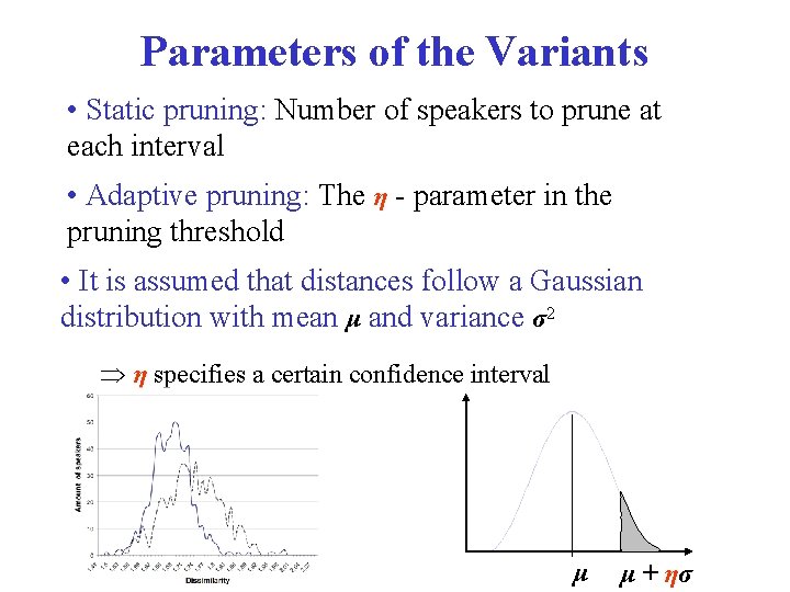
Parameters of the Variants • Static pruning: Number of speakers to prune at each interval • Adaptive pruning: The η - parameter in the pruning threshold • It is assumed that distances follow a Gaussian distribution with mean μ and variance σ2 η specifies a certain confidence interval μ μ + ησ

Experimental Setup TIMIT-corpus: • N = 630 American English speakers, clean speech • Sample rate Fs = 8 k. Hz, 16 bps resolution • Pre-processing and MFCC feature extraction : - Silence removed, pre-emphasis H(z) = 1 - 0. 97 z-1 - 30 ms Hamming window, shifted by 10 ms - 27 triangular bandpass filters spaced equally on mel-scale - 0 th cepstral coefficient excluded Speaker models : • Codebooks of 64 vectors by Linde-Buzo-Gray algorithm • Training data: 8. 8 seconds / speaker (without silence)

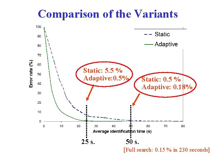
Evaluation Criteria • Identification error rate + Avg. identification time per speaker Combined: error rate as a function of time • Reference point: Full-search (no speaker pruning) achieves 0. 15 % error rate (one misclassified speaker) on average in 230 seconds ( 4 minutes)

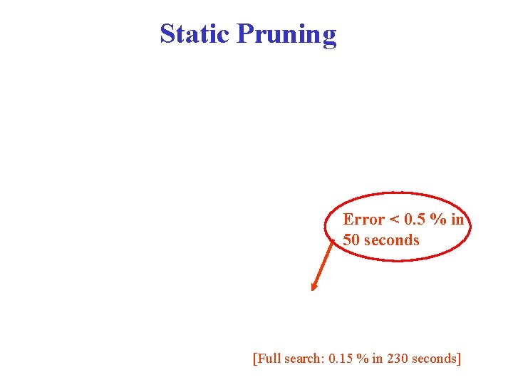
Static Pruning Error < 0. 5 % in 50 seconds [Full search: 0. 15 % in 230 seconds]

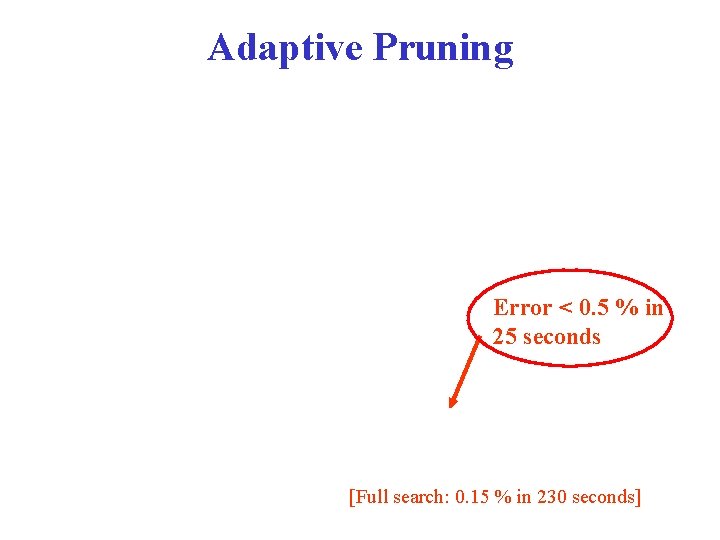
Adaptive Pruning Error < 0. 5 % in 25 seconds [Full search: 0. 15 % in 230 seconds]

Comparison of the Variants Static: 5. 5 % Adaptive: 0. 5% 25 s. Static: 0. 5 % Adaptive: 0. 18% 50 s. [Full search: 0. 15 % in 230 seconds]

Conclusions • Speed-up ratio 9: 1 with only minor degration in accuracy • Full search: 629/630 correct in 220 seconds • Static pruning: 595/630 correct in 25 seconds • Adaptive pruning: 627/630 correct in 25 seconds • Adaptive variant outperforms static variant • Selection of the parameters not crucial Easy to apply in practice • Both variants are straightforward to implement • Easily extendable to other models (e. g. GMM)