A Spatial Model of Social Interactions Multiplicity of

A Spatial Model of Social Interactions Multiplicity of Equilibria Pascal Mossay U of Reading, UK Pierre Picard U of Manchester, UK CORE, Louvain-la-Neuve Paris, July 2009

Agglomeration Economies • Increasing Returns (New Economic Geography) Market Mechanism • Social Interactions Non-Market Mechanism

Aim of the Paper • Social Interactions Desire of face-to-face contacts • Framework Communication Externality • Issues Emergence of Multiple Cities Shape and Spacing of Cities Market for Land

Related Literature • Beckmann (1976), Fujita & Thisse (2002) “Implication of Social Contacts on Shape of Cities” • Wang, Berliant, (2006, JET) “Only 1 Agglomeration in Equilibrium” • Fujita & Ogawa (1980, 1982, RSUE) “Multiple center configurations – Multiple Equilibria” • Hesley & Strange (2007, J. Econ. Geogr. ) “Endogenous Number of Social Contacts” • Tabuchi (1986, RSUE) “First best city is more concentrated than the eqm”

Plan of the Talk • • Spatial Interaction Model along a Circle Spatial Equilibria Characterization and Pareto-ranking First-best Distribution Robustness of Equilibria Local vs. Global Spatial Interactions

Spatial Interaction Model Beckmann (1976), Fujita and Thisse (2002) λ(x) x Space • Each agent located in x – Faces some residence cost – Benefits from face-to-face contacts with others – Faces some accessing cost

λ(x) Max U(z, s) z s r(x) λ(x) : consumption good : land consumption : rent in location x : population in location x A : social interaction benefit d(x, y): distance between x and y τ : travelling cost

Max U(z, s) = z + u(s) z, s, x z s r(x) λ(x) : consumption good : land consumption : rent in location x : population in location x A : social interaction benefit d(x, y): distance between x and y τ : travelling cost λ(x)

• Indirect Utility • Spatial Equilibrium • Trade-off Residence Cost Accessing Cost

Spatial Equilibrium λ(x) -a X=0 • Agents in x=-a: Low Residence Cost Agents in x=0 : High Residence Cost a High Accessing Cost Low Accessing Cost • Spatial Equilibrium: All agents achieve the same utility level • Distribution

Proposition: No Multiple-City Configuration City 1 City 2 City 3 x • Consider some agent in x By moving to his right, lower residence cost lower accessing cost Incentive to relocate

Spatial Interactions Along a Circle λ(x) • Agent density • Each agent - faces a residence cost - benefits from face-to-face contacts - faces an accessing cost

A priori: Many Possible Configurations City 2 City 1 City 3 Large & Small Cities City 3 Uneven Spacing

Characterization 1) Proposition: Cities can’t face each other “No Antipodal Cities” • At location x, by moving to the right marginal residence cost > 0 => Pop(east)> Pop(west) West x X+1/2 East • At location x+1/2, by moving clockwise marginal residence cost > 0 => Pop(west)> Pop(east)

Characterization 2) The number of Cities can’t be even P 1 P 4 x 1 P 2 • At location x 1: P 4=P 2+P 3 • At location x 3: P 4=P 1+P 2 x 4 • But then P 1=P 3 • Similarly, P 4=P 2 x 3 P 3 • Thus P 1=0

Characterization 3) Cities of equal size & evenly spaced • Proposition: An odd number of Equal & Evenly Spaced is a Spatial Equilibrium.

City 1 x City 2 City 3

x

x

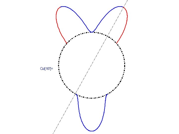
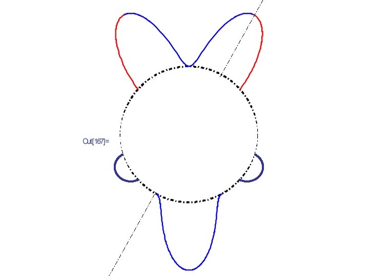
Robustness of Spatial Equilibria • Proposition: Spatial Adjustments towards higher utility neighborhoods leads back to eqm

Pareto-Ranking • Consider a Spatial Equilibrium with M cities V(M)= - (resid. Cost + intra-city cost + inter-city cost) decreases with M increases with M • V(M) decreases with M • Proposition: M=1 is the “best” equilibrium

Social Optimum First-Best Equilibrium

Social Optimum • In the decentralized equilibrium, agents do not internalize the other agents’ interaction cost [see Tabuchi (1986), Fujita-Thisse(2002)] • The Spatial Planner will build a city that is more concentrated than the equilibrium allocation

Localized Interactions (x-n, x+n) X-n x X+n • Consider an agent in location x moving to the right - faces a higher residence cost - gets closer to people at his right - further away from people at his left - gets access to “new” agents - looses access to some agents

Local vs Global Spatial Interactions Global Inter. Single Spatial Scale Local Inter. Multiple Spatial Scales

Conclusion • Along a circle, multiple cities emerge • Characterization: equal-size, evenly spaced • Pareto-ranking: 1 -city > 2 -city > 3 -city >… • Robustness wrt small initial perturbations • Local Interactions=>multiple spatial scales