A Simpler Minimum Spanning Tree Verification Algorithm Valerie

A Simpler Minimum Spanning Tree Verification Algorithm Valerie King Algorithmica, 18: 263– 270, 1997 D 94922004 陳冠宇 D 96945017 林振慶 R 96922013 黃于鳴 R 96922028 廖鳳玉 R 96922032 張瀠文 R 96922035 曾照涵 2008/05/22 1

Outline Introduction Borůvka Tree Property Komlós’s Algorithm for a Full Branching Tree Implementation Data Structures The Algorithm More Details Analysis Conclusion and Open Problems 2

Outline Introduction Borůvka Tree Property Komlós’s Algorithm for a Full Branching Tree Implementation Data Structures The Algorithm More Details Analysis Conclusion and Open Problems 3

Valerie King University of Victoria. Research interests: Randomized algorithms and data structures. Applications to networks and computational biology. Distributed computing. 4

Abstract Problem: Determine whether a given spanning tree in a graph is a minimal spanning tree. In 1984, Komlós presented an algorithm: A linear number of comparisons. But nonlinear overhead to determine which comparisons to make. This paper simplifies Komlós’s algorithm, and gives a linear time procedure using table lookup in the unit cost RAM model. 5

Related Works(1/2) Tarjan (1979) Path compression on balanced trees. O(m α(m, n)), almost linear running time. α(m, n) is a very slowly growing function. O(m) storage space. Komlós (1984) O(m) binary comparisons between edge costs. Non-linear time to determine which comparisons to make. 6

Related Works(2/2) Dixon, Rauch, and Tarjan (1992) O(m), linear time algorithm. Combines Tarjan’s almost-linear-time algorithm and Komlós’s algorithm, with a preprocessing and table-look-up method for small subproblems. Decompose the tree into a large subtree and many microtrees. Path compression (Tarjan 1979) is used on the large subtree. The comparison decision tree needed to implement Komlós’s strategy for each possible microtree is precomputed and stored in a table. Each microtree with its query paths is encoded. The table is used to loop up the appropriate comparisons to make. Model of computation: binary comparison, addition, substraction on edge cost on unit-cost random-access machine. 7

Definitions(1/3) A graph G = (V, E) with n nodes and m edges. A path of length k from x to y in G is a sequence of edges {x, v 1}, {v 1, v 2}, …, {vk-1, y}. A tree T = (V, E) is a graph such that T is connected and contains no cycles. T is a spanning tree if a tree is a subgraph of G with the same vertex set as T. 8

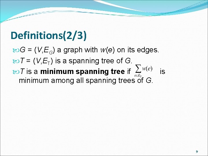
Definitions(2/3) G = (V, EG) a graph with w(e) on its edges. T = (V, ET) is a spanning tree of G. T is a minimum spanning tree if is minimum among all spanning trees of G. 9

Definitions(3/3) T(x, y): the set of edges in the path in a tree T from node x to node y. In a tree T, there is a unique path from x to y. A rooted tree is a tree with a distinguished node called root. A Full branching tree is a rooted tree with all leaves on the same level and each internal node having at least two children. B(x, y): the set of edges in the path in a full branching tree B from leaf x to leaf y. 10

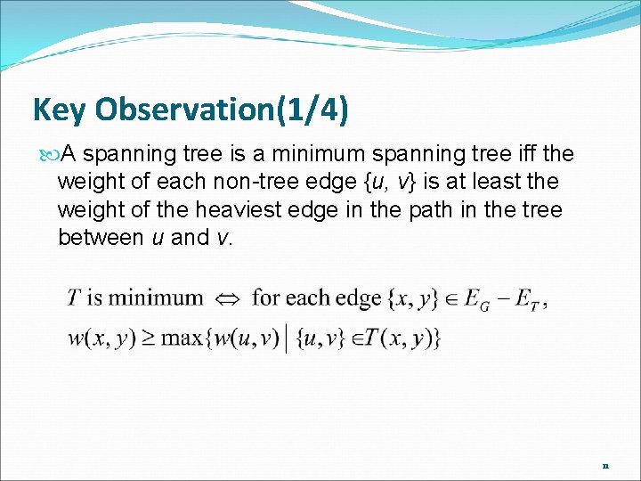
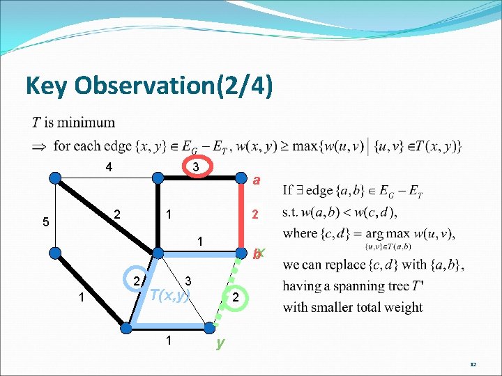
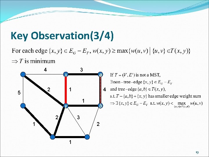
Key Observation(1/4) A spanning tree is a minimum spanning tree iff the weight of each non-tree edge {u, v} is at least the weight of the heaviest edge in the path in the tree between u and v. 11

Key Observation(2/4) 4 3 2 5 a 1 42 1 bx 3 T(x, y) 1 2 y 12

Key Observation(3/4) 4 x 2 5 3 a 1 4 1 y 2 b 3 1 2 1 13

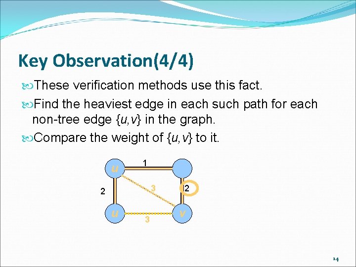
Key Observation(4/4) These verification methods use this fact. Find the heaviest edge in each such path for each non-tree edge {u, v} in the graph. Compare the weight of {u, v} to it. u 1 3 2 u 3 2 v 14

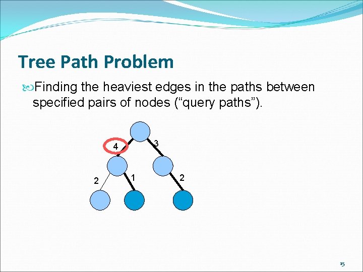
Tree Path Problem Finding the heaviest edges in the paths between specified pairs of nodes (“query paths”). 3 4 2 15

Main Ideas(1/2) T is a spanning tree. A simple O(n) algorithm to construct a full branching tree B with no more than 2 n edges. The weight of the heaviest edge in T(x, y) is the weight of the heaviest edge in B(x, y). Use the version of the Komlós’s algorithm for full branching trees. Much simpler than his algorithm for general trees. 16

Main Ideas(2/2) Linear time implementation using table lookup of a few simple functions. Can be constructed in time linear in the size of the tree. Model of computation: unit random access model with word size θ(log n) bits. Allow edge weights to be compared, added, or subtracted at unit cost. 17

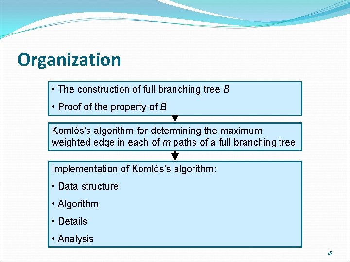
Organization • The construction of full branching tree B • Proof of the property of B Komlós’s algorithm for determining the maximum weighted edge in each of m paths of a full branching tree Implementation of Komlós’s algorithm: • Data structure • Algorithm • Details • Analysis 18

Outline Introduction Borůvka Tree Property Komlós’s Algorithm for a Full Branching Tree Implementation Data Structures The Algorithm More Details Analysis Conclusion and Open Problems 19

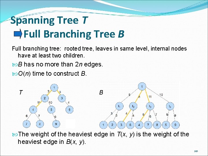
Spanning Tree T Full Branching Tree B Full branching tree: rooted tree, leaves in same level, internal nodes have at least two children. B has no more than 2 n edges. O(n) time to construct B. T B The weight of the heaviest edge in T(x, y) is the weight of the heaviest edge in B(x, y). 20

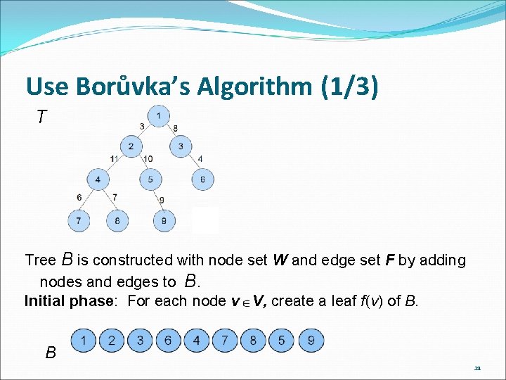
Use Borůvka’s Algorithm (1/3) T Tree B is constructed with node set W and edge set F by adding nodes and edges to B. Initial phase: For each node v V, create a leaf f(v) of B. B 21

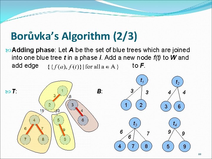
Borůvka’s Algorithm (2/3) Adding phase: Let A be the set of blue trees which are joined into one blue tree t in a phase i. Add a new node f(t) to W and add edge to F. t 1 T: 3 B: 1 t 2 3 2 4 3 6 t 4 t 3 6 4 6 7 4 7 9 8 5 9 9 22

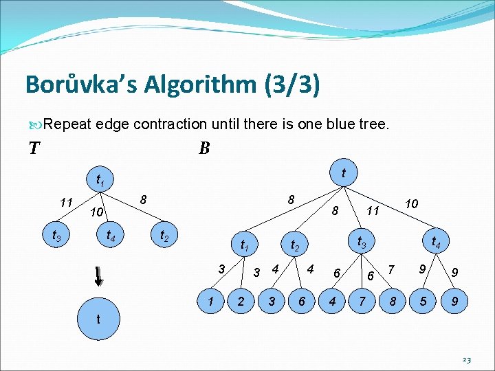
Borůvka’s Algorithm (3/3) Repeat edge contraction until there is one blue tree. T B t t 1 11 8 10 t 3 t 4 8 t 2 t 1 3 1 8 2 3 4 6 t 4 t 3 t 2 3 4 10 11 6 4 6 7 7 9 9 8 5 9 t 23

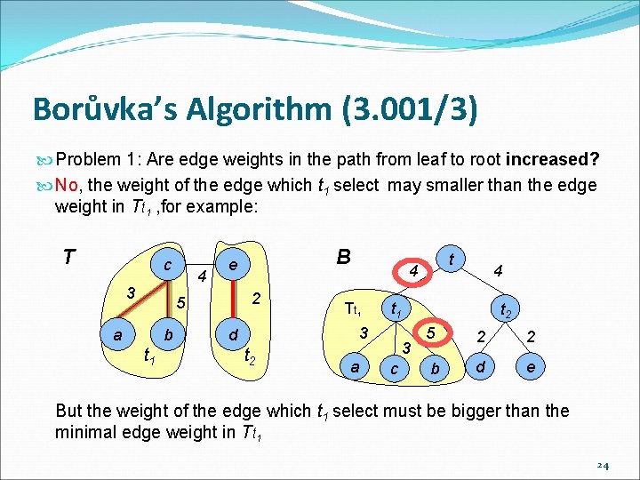
Borůvka’s Algorithm (3. 001/3) Problem 1: Are edge weights in the path from leaf to root increased? No, the weight of the edge which t 1 select may smaller than the edge weight in Tt 1 , for example: T c 3 4 2 5 a b t 1 B e Tt 1 t 2 a 4 t 1 3 d t 4 3 c t 2 5 2 2 b d e But the weight of the edge which t 1 select must be bigger than the minimal edge weight in Tt 1 24

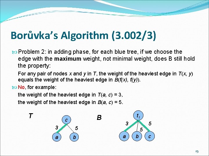
Borůvka’s Algorithm (3. 002/3) Problem 2: in adding phase, for each blue tree, if we choose the edge with the maximum weight, not minimal weight, does B still hold the property: For any pair of nodes x and y in T, the weight of the heaviest edge in T(x, y) equals the weight of the heaviest edge in B(f(x), f(y)). No, for example: the weight of the heaviest edge in T(a, c) = 3, the weight of the heaviest edge in B(a, c) = 5. T B c 3 a 5 b t 1 5 3 5 a b c 25

Borůvka’s Tree Property (1/5) The number of blue trees drops by a factor of at least two after each phase. B is a full branching tree. Theorem 1 For any pair of nodes x and y in T, the weight of the heaviest edge in T(x, y) equals the weight of the heaviest edge in B(f(x), f(y)). 26

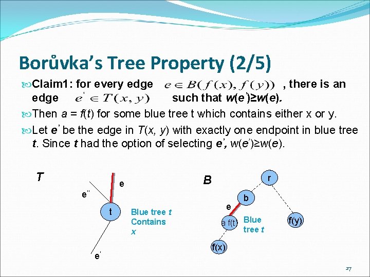
Borůvka’s Tree Property (2/5) Claim 1: for every edge , there is an edge such that w(e’)≥w(e). Then a = f(t) for some blue tree t which contains either x or y. Let e’ be the edge in T(x, y) with exactly one endpoint in blue tree t. Since t had the option of selecting e’, w(e’)≥w(e). T r B e e’’ t e’ Blue tree t Contains x e b a f(t) Blue tree t f(y) f(x) 27

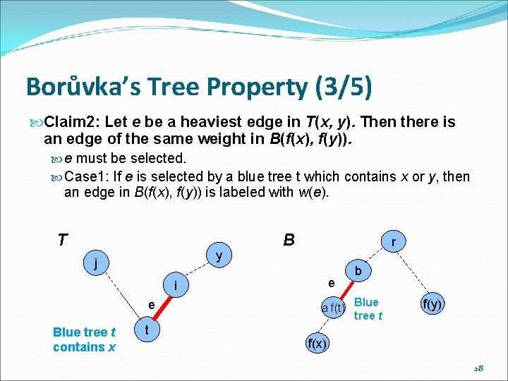
Borůvka’s Tree Property (3/5) Claim 2: Let e be a heaviest edge in T(x, y). Then there is an edge of the same weight in B(f(x), f(y)). e must be selected. Case 1: If e is selected by a blue tree t which contains x or y, then an edge in B(f(x), f(y)) is labeled with w(e). T y j B r e i e Blue tree t contains x t b a f(t) Blue tree t f(y) f(x) 28

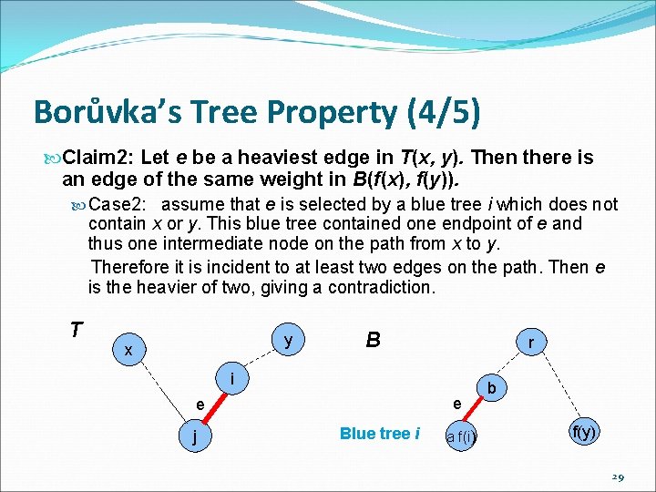
Borůvka’s Tree Property (4/5) Claim 2: Let e be a heaviest edge in T(x, y). Then there is an edge of the same weight in B(f(x), f(y)). Case 2: assume that e is selected by a blue tree i which does not contain x or y. This blue tree contained one endpoint of e and thus one intermediate node on the path from x to y. Therefore it is incident to at least two edges on the path. Then e is the heavier of two, giving a contradiction. T y x B r i e e j Blue tree i a f(i) b f(y) 29

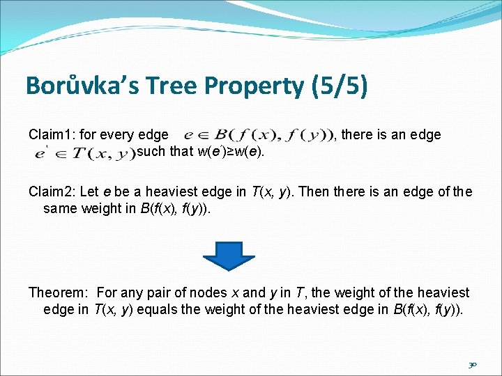
Borůvka’s Tree Property (5/5) Claim 1: for every edge such that w(e’)≥w(e). , there is an edge Claim 2: Let e be a heaviest edge in T(x, y). Then there is an edge of the same weight in B(f(x), f(y)). Theorem: For any pair of nodes x and y in T, the weight of the heaviest edge in T(x, y) equals the weight of the heaviest edge in B(f(x), f(y)). 30

Outline Introduction Borůvka Tree Property Komlós’s Algorithm for a Full Branching Tree Implementation Data Structures The Algorithm More Details Analysis Conclusion and Open Problems 31

MST Verification Using Full Branching Tree Given a spanning tree T of a graph G. Construct a full branching tree B from T using Borůvka’s algorithm. For every non-tree edge e = {u, v} in G, find the heaviest edge e’ in the query path B(f(u), f(v)), and see if w(e) ≥ w(e’) or not. By Borůvka’s tree property. If for all non-tree edge e, w(e) ≥ w(e’), then T is a minimum spanning tree of G. 32

Komlós’s Algorithm (1/5) Given a full branching tree with n nodes and m query paths between pairs of leaves, Komlós’s algorithm can compute the heaviest edge in every query path using only linear number of comparisons. For each query path (leaf x -> leaf y), break up the path into two half-paths from leaf up to the lowest common ancestor of the pair. Find the heaviest edge in each half-path and compare the two edges to determine the heaviest edge in the whole path. 33

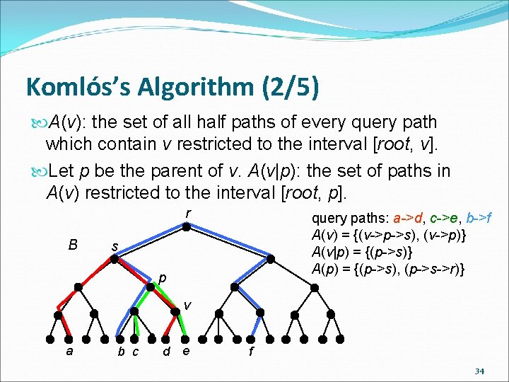
Komlós’s Algorithm (2/5) A(v): the set of all half paths of every query path which contain v restricted to the interval [root, v]. Let p be the parent of v. A(v|p): the set of paths in A(v) restricted to the interval [root, p]. r B query paths: a->d, c->e, b->f A(v) = {(v->p->s), (v->p)} A(v|p) = {(p->s)} A(p) = {(p->s), (p->s->r)} s p v a b c d e f 34

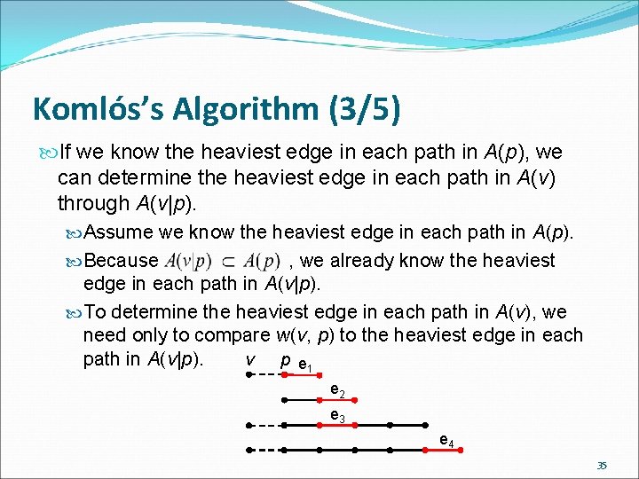
Komlós’s Algorithm (3/5) If we know the heaviest edge in each path in A(p), we can determine the heaviest edge in each path in A(v) through A(v|p). Assume we know the heaviest edge in each path in A(p). Because , we already know the heaviest edge in each path in A(v|p). To determine the heaviest edge in each path in A(v), we need only to compare w(v, p) to the heaviest edge in each path in A(v|p). v p e 1 e 2 e 3 e 4 35

Komlós’s Algorithm (4/5) Starting from the root, descend level by level and as each node v encountered, the heaviest edge in each path in A(v) can be determined. For a query path(x->y), use A(x) and A(y) to determine the heaviest edge in each half path, and compare the two to determine the heaviest edge in the query path. 36

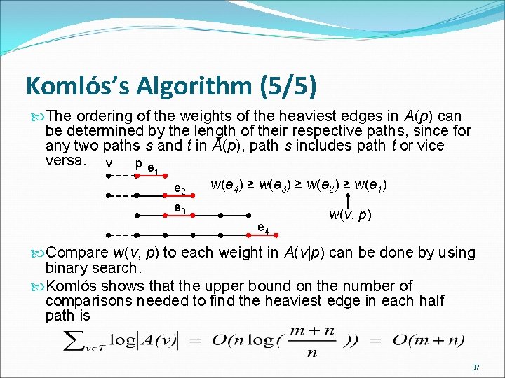
Komlós’s Algorithm (5/5) The ordering of the weights of the heaviest edges in A(p) can be determined by the length of their respective paths, since for any two paths s and t in A(p), path s includes path t or vice versa. v pe 1 e 2 w(e 4) ≥ w(e 3) ≥ w(e 2) ≥ w(e 1) e 3 e 4 w(v, p) Compare w(v, p) to each weight in A(v|p) can be done by using binary search. Komlós shows that the upper bound on the number of comparisons needed to find the heaviest edge in each half path is 37

Outline Introduction Borůvka Tree Property Komlós’s Algorithm for a Full Branching Tree Implementation Data Structures The Algorithm More Details Analysis Conclusion and Open Problems 38

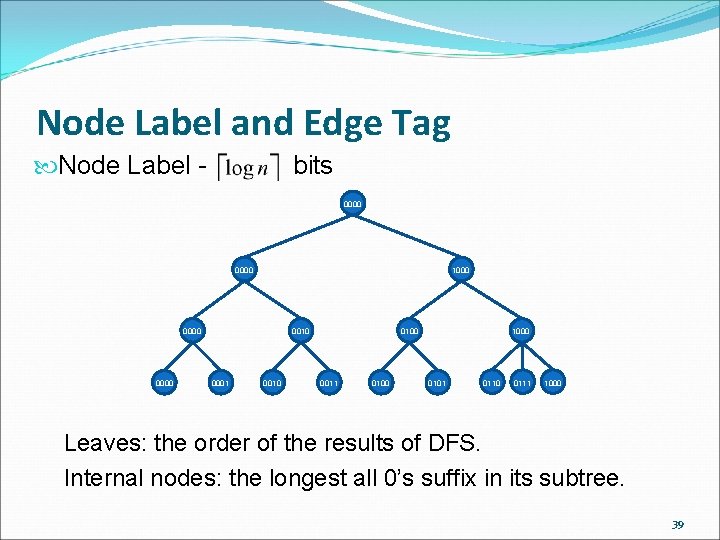
Node Label and Edge Tag Node Label - bits 0000 1000 0000 0010 0001 0010 0100 0011 0100 1000 0101 0110 0111 1000 Leaves: the order of the results of DFS. Internal nodes: the longest all 0’s suffix in its subtree. 39

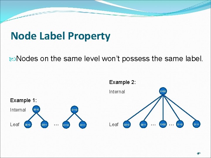
Node Label Property Nodes on the same level won’t possess the same label. Example 2: Internal 0100 Example 1: Internal Leaf 0010 0110 0011 … 0110 0111 Leaf 0010 0011 … 0100 … 0110 0111 40

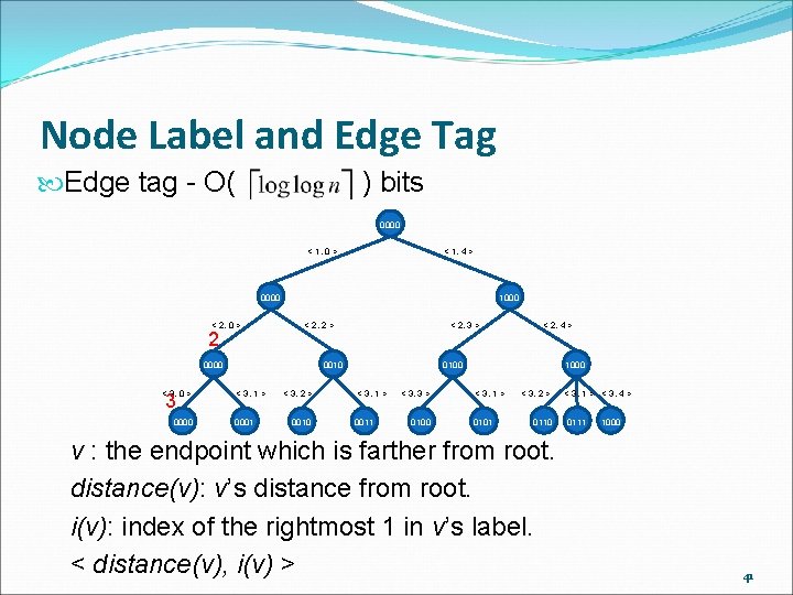
Node Label and Edge Tag Edge tag - O( ) bits 0000 < 1, 0 > < 1, 4 > 0000 < 2, 0 > 2 1000 < 2, 2 > 0000 < 3, 0 > 3 0000 < 2, 3 > 0010 < 3, 1 > 0001 < 3, 2 > 0010 < 2, 4 > 0100 < 3, 1 > 0011 < 3, 3 > 0100 1000 < 3, 1 > 0101 < 3, 2 > 0110 v : the endpoint which is farther from root. distance(v): v’s distance from root. i(v): index of the rightmost 1 in v’s label. < distance(v), i(v) > < 3, 1 > < 3, 4 > 0111 1000 41

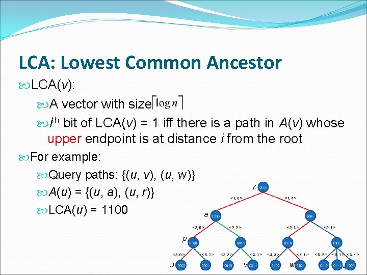
LCA: Lowest Common Ancestor LCA(v): A vector with size ith bit of LCA(v) = 1 iff there is a path in A(v) whose upper endpoint is at distance i from the root For example: Query paths: {(u, v), (u, w)} r A(u) = {(u, a), (u, r)} LCA(u) = 1100 a p u v w 43

Big. Lists and Small. Lists (1/3) If |A(v)| > wordsize / tagsize , |A(v)| is Big Otherwise, |A(v)| is Small 44

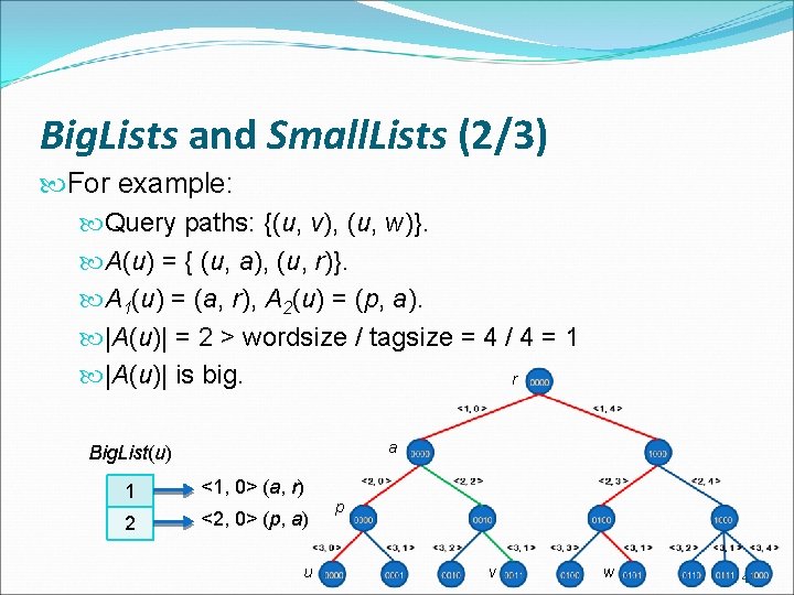
Big. Lists and Small. Lists (2/3) For example: Query paths: {(u, v), (u, w)}. A(u) = { (u, a), (u, r)}. A 1(u) = (a, r), A 2(u) = (p, a). |A(u)| = 2 > wordsize / tagsize = 4 / 4 = 1 |A(u)| is big. r a Big. List(u) 1 <1, 0> (a, r) 2 <2, 0> (p, a) u p v w 45

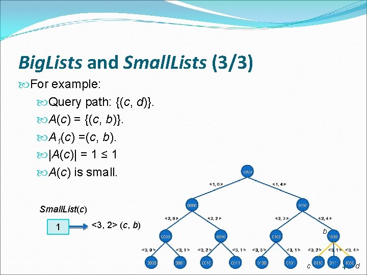
Big. Lists and Small. Lists (3/3) For example: Query path: {(c, d)}. A(c) = {(c, b)}. A 1(c) =(c, b). |A(c)| = 1 ≤ 1 A(c) is small. Small. List(c) 1 <3, 2> (c, b) b c 46 d

Outline Introduction Borůvka Tree Property Komlós’s Algorithm for a Full Branching Tree Implementation Data Structures The Algorithm More Details Analysis Conclusion and Open Problems 47

Goal of the Algorithm Generate big. List(v) or small. List(v) in time proportional to log|A(v)|. The time spent implementing Komlós’s algorithm at each node does not exceed the worst case number of comparisons needed at each node. 48

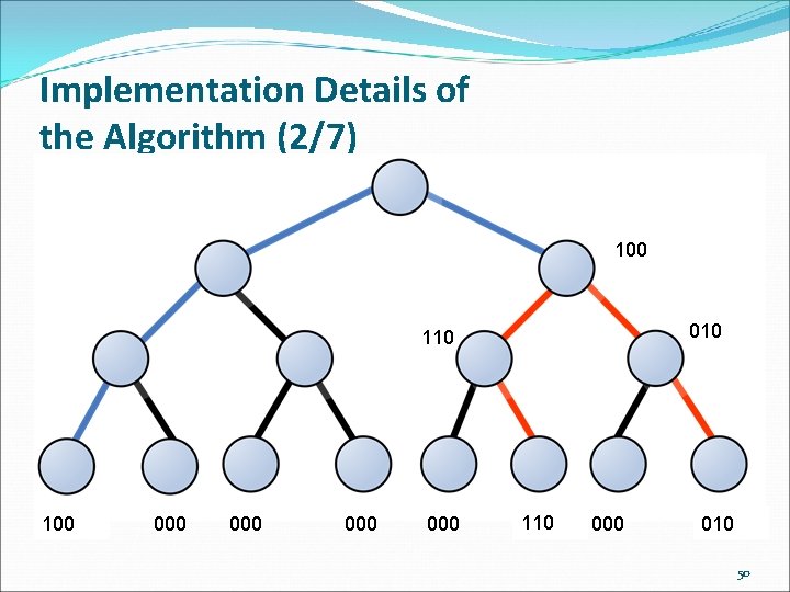
Implementation Details of the Algorithm (1/7) The computation of the LCAs. Compute all LCAs for each pair of endpoints of the m query paths. Form the vector LCA(l) for each leaf l. Form the vector LCA(v) for a node at distance i from the root by ORing together the LCAs of its children and setting the jth bits to 0 for all j≧i. Compute all LCAs for each pair of endpoints of the m query paths using an algorithm that runs in time O(n + m). 49

Implementation Details of the Algorithm (2/7) 100 010 100 000 000 000 110 000 100 000 010 50

Implementation Details of the Algorithm (3/7) Subword tagsize bits: loglogn. Swnum The maximum number of subwords stored in a word. 51

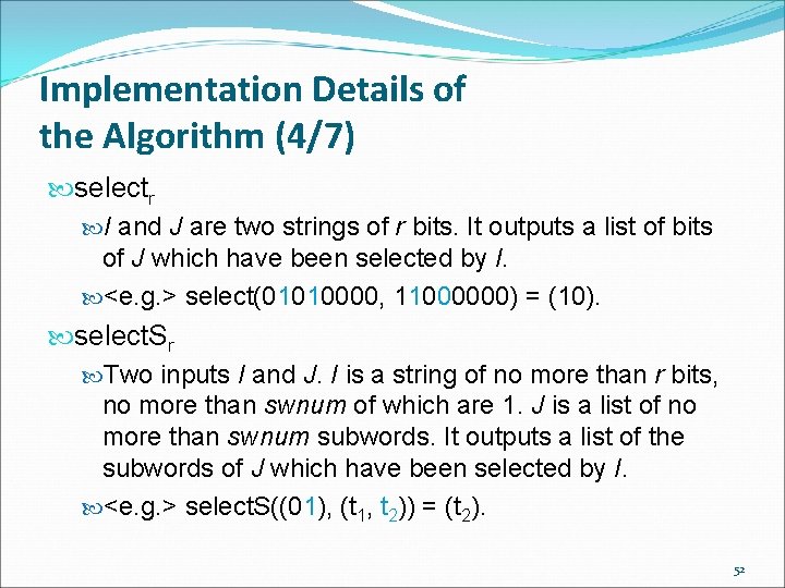
Implementation Details of the Algorithm (4/7) selectr I and J are two strings of r bits. It outputs a list of bits of J which have been selected by I. <e. g. > select(01010000, 11000000) = (10). select. Sr Two inputs I and J. I is a string of no more than r bits, no more than swnum of which are 1. J is a list of no more than swnum subwords. It outputs a list of the subwords of J which have been selected by I. <e. g. > select. S((01), (t 1, t 2)) = (t 2). 52

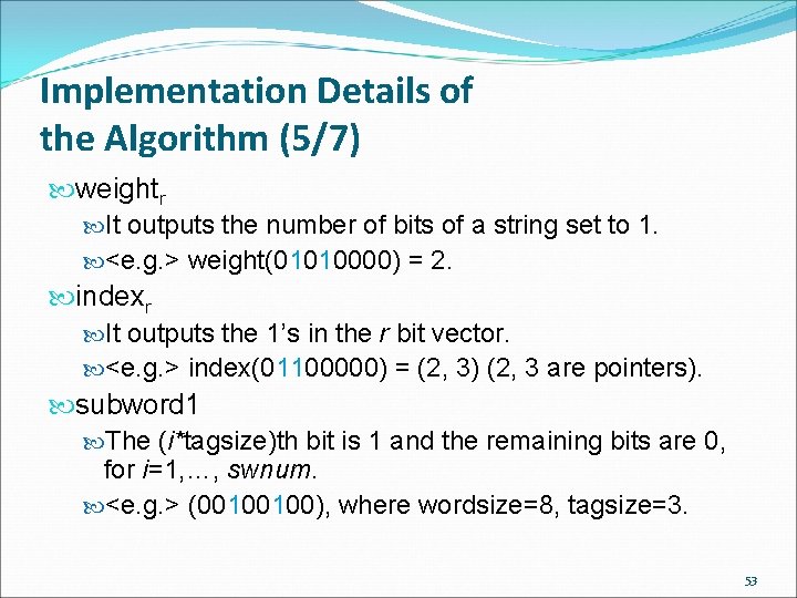
Implementation Details of the Algorithm (5/7) weightr It outputs the number of bits of a string set to 1. <e. g. > weight(01010000) = 2. indexr It outputs the 1’s in the r bit vector. <e. g. > index(01100000) = (2, 3) (2, 3 are pointers). subword 1 The (i*tagsize)th bit is 1 and the remaining bits are 0, for i=1, …, swnum. <e. g. > (00100100), where wordsize=8, tagsize=3. 53

Implementation Details of the Algorithm (6/7) To implement these operations, we need to preprocess a few functions so that we may do table lookup of these functions. When the size of the input is no greater than logn+c, where c is a constant, the preprocessing time is O(n). 54

Implementation Details of the Algorithm (7/7) We cannot afford to build a table for selectwordsize and select. Swordsize which takes inputs of 2 wordsize bits, since the table would be too large. However, we can compute these functions as needed in constant time using table lookups of those functions on input size wordsize/2. A table for all inputs of length r can be built by first building a table for inputs of size r/2, looking up the result for the two halves, and, in constant time, putting the results together to form the entry. 55

Outline Introduction Borůvka Tree Property Komlós’s Algorithm for a Full Branching Tree Implementation Data Structures The Algorithm More Details Analysis Conclusion and Open Problems 56

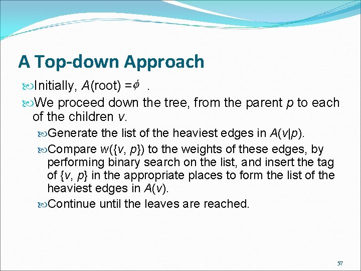
A Top-down Approach Initially, A(root) =. We proceed down the tree, from the parent p to each of the children v. Generate the list of the heaviest edges in A(v|p). Compare w({v, p}) to the weights of these edges, by performing binary search on the list, and insert the tag of {v, p} in the appropriate places to form the list of the heaviest edges in A(v). Continue until the leaves are reached. 57

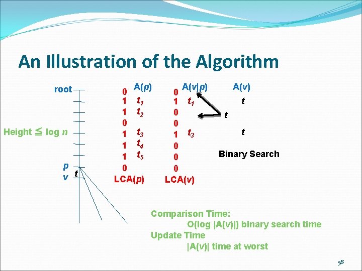
An Illustration of the Algorithm root Height ≦ log n p v t A(p) 0 1 t 1 1 t 2 0 1 t 3 1 t 4 1 t 5 0 LCA(p) A(v|p) 0 1 t 1 0 0 1 t 3 0 0 0 LCA(v) t t t Binary Search Comparison Time: O(log |A(v)|) binary search time Update Time |A(v)| time at worst 58

A Preliminary Analysis We got a naïve time algorithm. Observe that only comparisons are used, but with a non-linear time overhead to maintain the list. A linear time algorithm for this problem in a pointer machine is not thought possible. (such a result would imply a linear-time algorithm for computing LCA in a pointer machine) Our Goal: Give a linear time implementation in the unit cost RAM model, in which an O(log n) operation can be done in constant time. 59

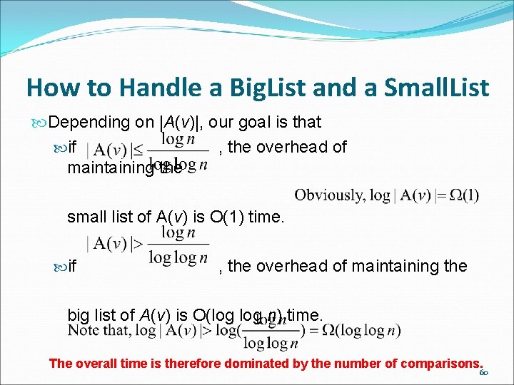
How to Handle a Big. List and a Small. List Depending on |A(v)|, our goal is that if , the overhead of maintaining the small list of A(v) is O(1) time. if , the overhead of maintaining the big list of A(v) is O(log n) time. The overall time is therefore dominated by the number of comparisons. 60

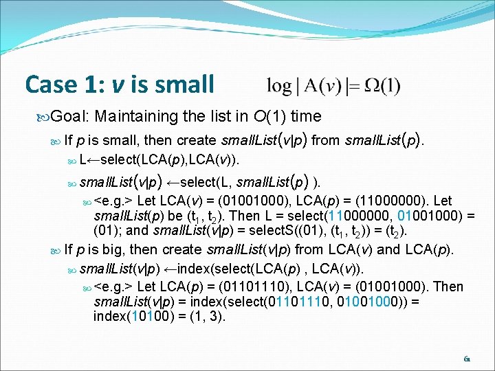
Case 1: v is small Goal: Maintaining the list in O(1) time p is small, then create small. List(v|p) from small. List(p). L←select(LCA(p), LCA(v)). If small. List (v|p) ←select(L, small. List(p) ). <e. g. > Let LCA(v) = (01001000), LCA(p) = (11000000). Let small. List(p) be (t 1, t 2). Then L = select(11000000, 01001000) = (01); and small. List(v|p) = select. S((01), (t 1, t 2)) = (t 2). If p is big, then create small. List(v|p) from LCA(v) and LCA(p). small. List(v|p) ←index(select(LCA(p) , LCA(v)). <e. g. > Let LCA(p) = (01101110), LCA(v) = (01001000). Then small. List(v|p) = index(select(01101110, 01001000)) = index(10100) = (1, 3). 61

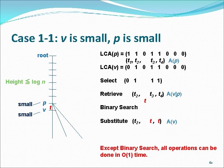
Case 1 -1: v is small, p is small root Height ≦ log n LCA(p) = (1 1 0 0 0) (t 1, t 2 , t 3 , t 4) A(p) LCA(v) = (0 1 1 0 0 0) Select Retrieve small p v t (0 1 (t 2 , 1 1) t t 3 , t 4) A(v|p) Binary Search Substitute (t 2 , t , t) A(v) Except Binary Search, all operations can be done in O(1) time. 62

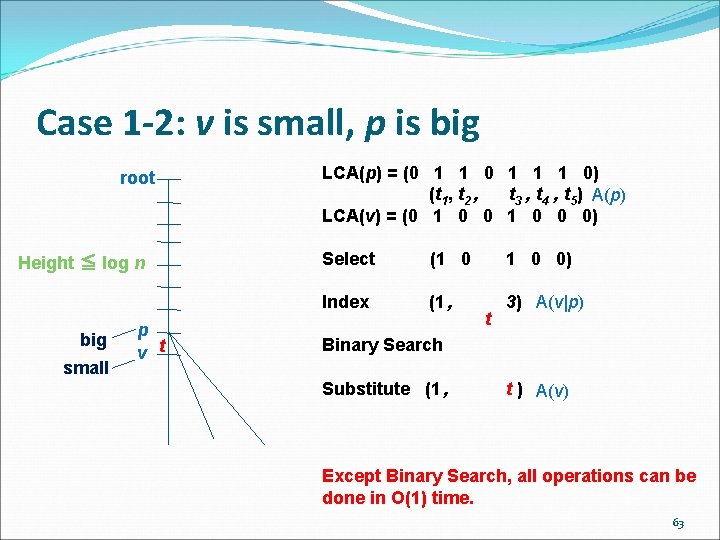
Case 1 -2: v is small, p is big root Height ≦ log n big small p v t LCA(p) = (0 1 1 1 0) (t 1, t 2 , t 3 , t 4 , t 5) A(p) LCA(v) = (0 1 0 0 0) Select (1 0 0) Index (1 , 3) A(v|p) t Binary Search Substitute (1 , t ) A(v) Except Binary Search, all operations can be done in O(1) time. 63

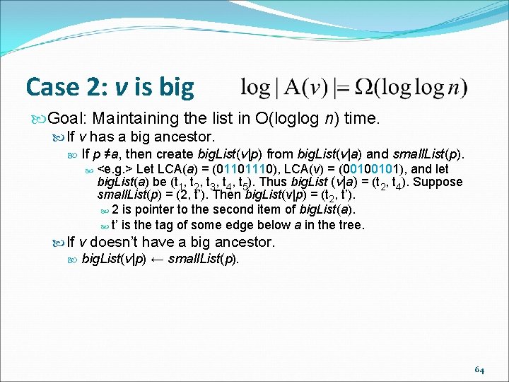
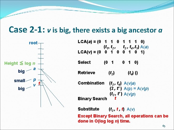
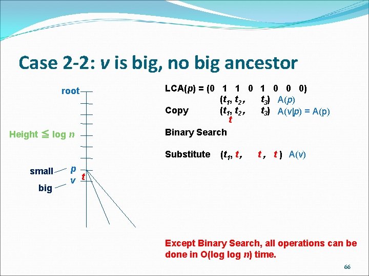
Case 2: v is big Goal: Maintaining the list in O(loglog n) time. If v has a big ancestor. If p ≠a, then create big. List(v|p) from big. List(v|a) and small. List(p). <e. g. > Let LCA(a) = (01101110), LCA(v) = (00100101), and let big. List(a) be (t 1, t 2, t 3, t 4, t 5). Thus big. List (v|a) = (t 2, t 4). Suppose small. List(p) = (2, t’). Then big. List(v|p) = (t 2, t’). 2 is pointer to the second item of big. List(a). t’ is the tag of some edge below a in the tree. If v doesn’t have a big ancestor. big. List(v|p) ← small. List(p). 64

Case 2 -1: v is big, there exists a big ancestor a root Height ≦ log n a big small big p v t LCA(a) = (0 1 1 1 0) (t 1, t 2 , t 3 , t 4 , t 5) A(a) LCA(v) = (0 0 1 0 1) Select (0 1 0) (t 2) (t 4) () Retrieve Combination (t 2 , t 4) A(v|a) (2 , t’ ) A(p) = A(v|p) (t 2 , t’ ) A(v|p) t Binary Search Substitute (t 2 , t) A(v) Except Binary Search, all operations can be done in O(log n) time. 65

Case 2 -2: v is big, no big ancestor root Height ≦ log n LCA(p) = (0 1 1 0 0 0) (t 1, t 2 , t 3) A(p) Copy (t 1, t 2 , t 3) A(v|p) = A(p) t Binary Search Substitute small big (t 1, t , t ) A(v) p v t Except Binary Search, all operations can be done in O(log n) time. 66

Outline Introduction Borůvka Tree Property Komlós’s Algorithm for a Full Branching Tree Implementation Data Structures The Algorithm More Details Analysis Conclusion and Open Problems 67

Time Complexity Preparation time: LCA query problem: O(m + n) time. Table lookup approach for O(log n)-bit operations: O(n) time. The overhead for each case does not exceed O(log |A(v)|) time, which leads to an time for maintaining the list. Compare the heaviest edges in each half-paths with the weight of each non-tree edge: O(m) time. Overall time complexity is O(m + n) time. 68

Outline Introduction Borůvka Tree Property Komlós’s Algorithm for a Full Branching Tree Implementation Data Structures The Algorithm More Details Analysis Conclusion and Open Problems 69

Conclusions and Open Problems The paper reduces Komlós’s algorithm to the simpler case of the full branching tree, and gives an algorithm with linear-time overhead for its implementation in the unit cost RAM. Some open problems remain: Give a linear time algorithm for the MST verification problem in a pointer machine. The tree-path problem: Given a static tree, preprocess it so that one can quickly retrieve the heaviest path in any online query path. 70

Thank You 71