A Simple Model for Analyzing P 2 P

A Simple Model for Analyzing P 2 P Streaming Protocols Zhou Yipeng Chiu Dah. Ming John, C. S. Lui The Chinese University of Hong Kong

Outline l l Introduction Model & Chunk Selection Strategies Simulation Conclusion

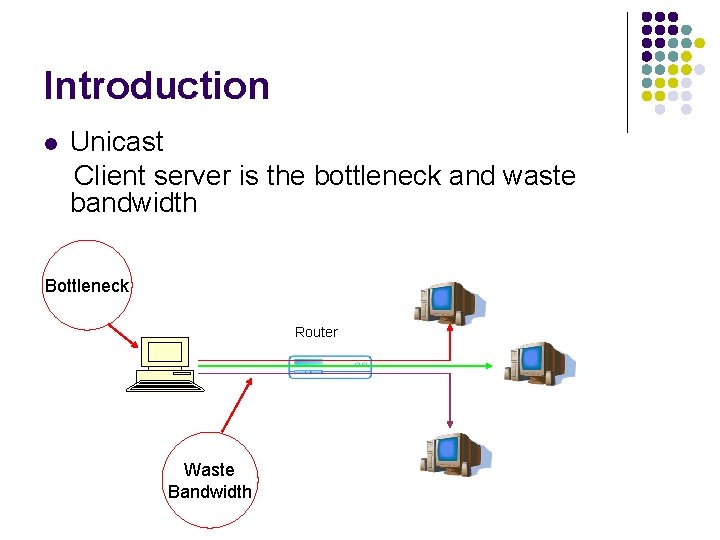
Introduction l Unicast Client server is the bottleneck and waste bandwidth Bottleneck Router Waste Bandwidth

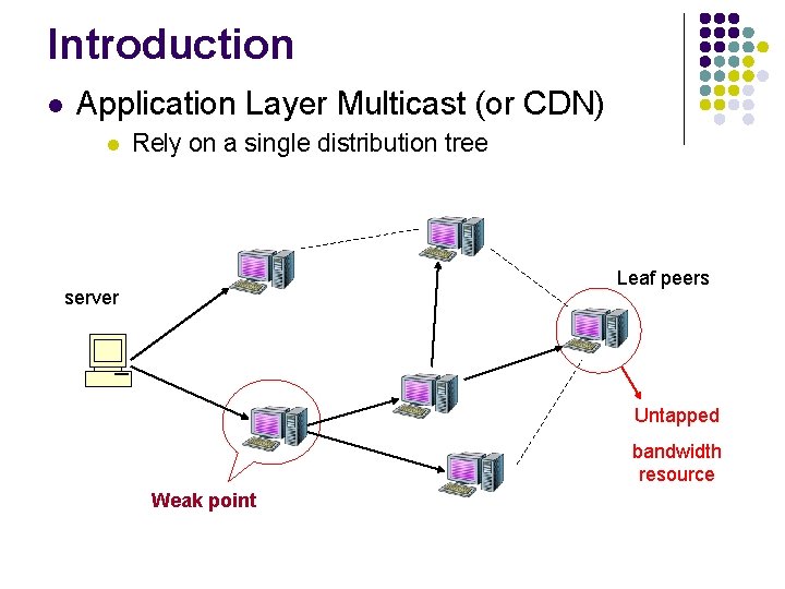
Introduction l Application Layer Multicast (or CDN) l Rely on a single distribution tree Leaf peers server Untapped bandwidth resource Weak point

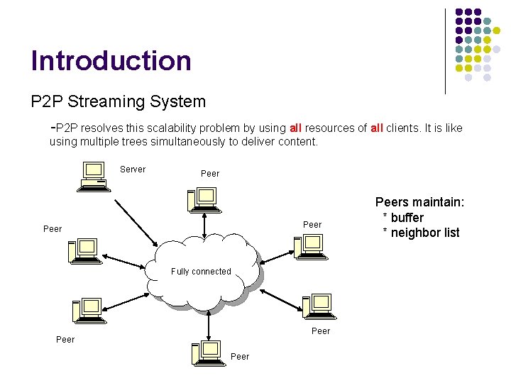
Introduction P 2 P Streaming System -P 2 P resolves this scalability problem by using all resources of all clients. It is like using multiple trees simultaneously to deliver content. Server Peer Fully connected Peers maintain: * buffer * neighbor list

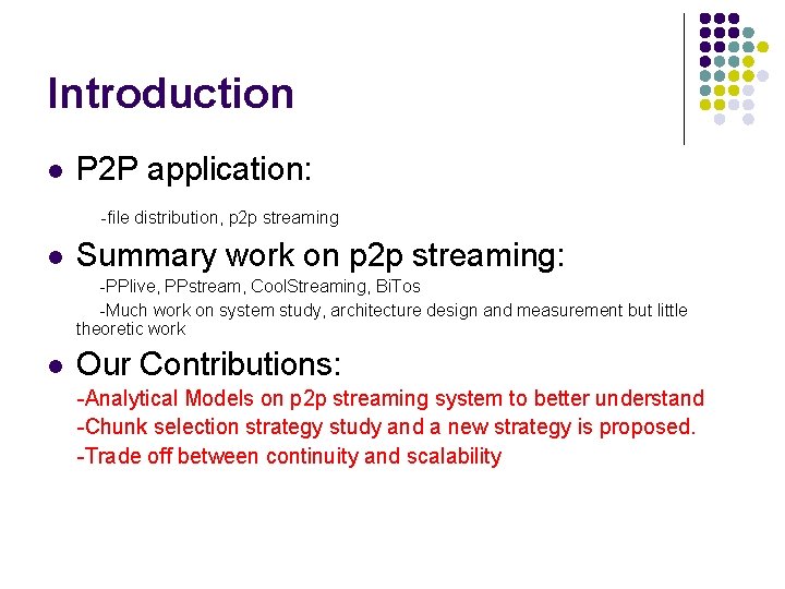
Introduction l P 2 P application: -file distribution, p 2 p streaming l Summary work on p 2 p streaming: -PPlive, PPstream, Cool. Streaming, Bi. Tos -Much work on system study, architecture design and measurement but little theoretic work l Our Contributions: -Analytical Models on p 2 p streaming system to better understand -Chunk selection strategy study and a new strategy is proposed. -Trade off between continuity and scalability

Outline l l Introduction Model & Chunk Selection Strategies Simulation Conclusion

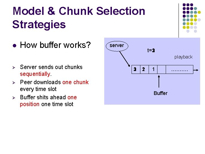
Model & Chunk Selection Strategies l How buffer works? server t=1 t=2 t=3 playback Ø Ø Ø Server sends out chunks sequentially. Peer downloads one chunk every time slot Buffer shits ahead one position one time slot 1 2 3 1 2 1 Buffer ……….

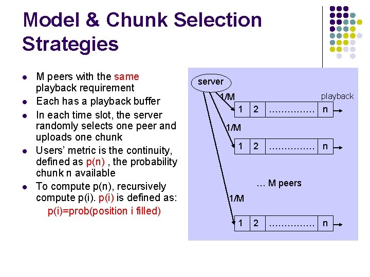
Model & Chunk Selection Strategies l l l M peers with the same playback requirement Each has a playback buffer In each time slot, the server randomly selects one peer and uploads one chunk Users’ metric is the continuity, defined as p(n) , the probability chunk n available To compute p(n), recursively compute p(i) is defined as: p(i)=prob(position i filled) server playback 1/M 1 2 …………… n 1/M 1 … M peers 1/M 1 2 …………… n

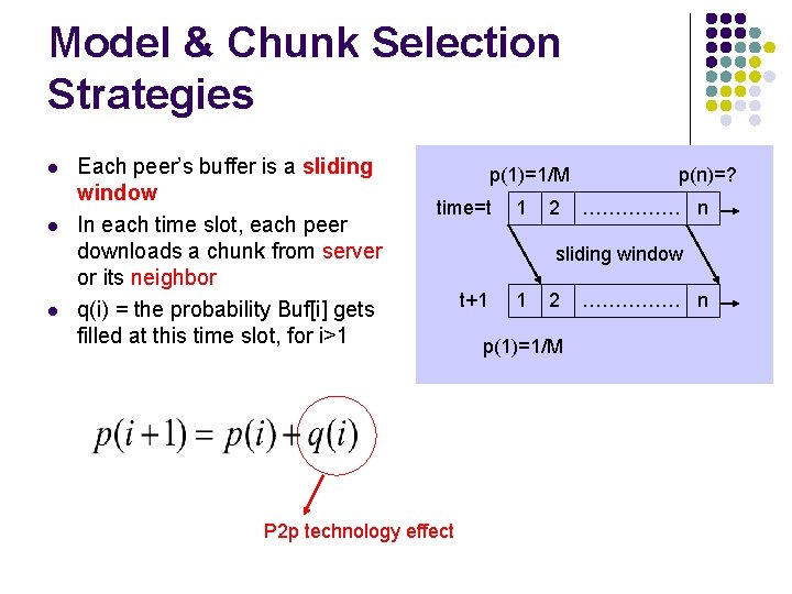
Model & Chunk Selection Strategies l l l Each peer’s buffer is a sliding window In each time slot, each peer downloads a chunk from server or its neighbor q(i) = the probability Buf[i] gets filled at this time slot, for i>1 p(1)=1/M time=t P 2 p technology effect 1 2 p(n)=? …………… n sliding window t+1 1 2 p(1)=1/M …………… n

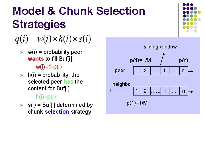
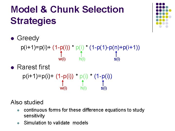
Model & Chunk Selection Strategies Ø Ø Ø w(i) = probability peer wants to fill Buf[i] w(i)=1 -p(i) h(i) = probability the selected peer has the content for Buf[i] h(i)=p(i) s(i) = Buf[i] determined by chunk selection strategy sliding window p(1)=1/M peer p(n) 1 2 …… i … n 1 2. …. . i … neighbo r p(1)=1/M n

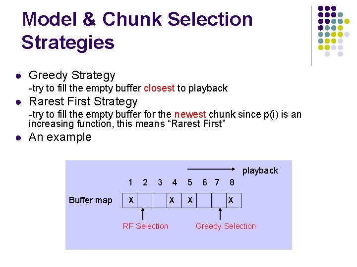
Model & Chunk Selection Strategies l Greedy Strategy -try to fill the empty buffer closest to playback l Rarest First Strategy -try to fill the empty buffer for the newest chunk since p(i) is an increasing function, this means “Rarest First” l An example playback 1 Buffer map 2 3 X RF Selection 4 5 X X 6 7 8 X Greedy Selection

Model & Chunk Selection Strategies l Greedy p(i+1)=p(i)+ (1 -p(i)) * p(i) * (1 -p(1)-p(n)+p(i+1)) w(i) l h(i) s(i) Rarest first p(i+1)=p(i)+ (1 -p(i)) * p(i) * (1 -p(i)) w(i) h(i) s(i) Also studied l l continuous forms for these difference equations to study sensitivity Simulation to validate models

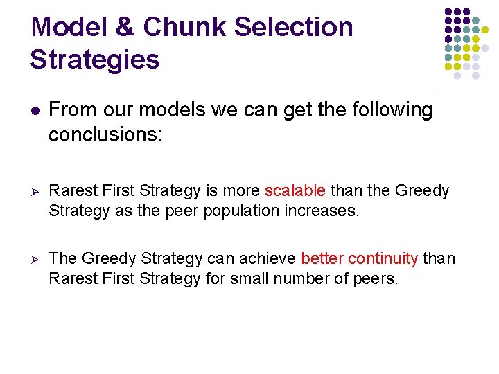
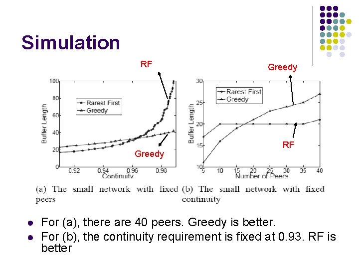
Model & Chunk Selection Strategies l From our models we can get the following conclusions: Ø Rarest First Strategy is more scalable than the Greedy Strategy as the peer population increases. Ø The Greedy Strategy can achieve better continuity than Rarest First Strategy for small number of peers.

A New Chunk Selection Strategy l Ø Ø Partition the buffer into [1, m] and [m+1, n] Use RF for [1, m] first If no chunks available for download by RF, use Greedy for [m+1, n] Buffer map 1 ……. . m m+1. . ……… n First do RF l Second do Greedy Difference equations become for i = 1, …, m-1 for i = m, … n-1

Outline l l Introduction Model & Chunk Selection Strategies Simulation Conclusion

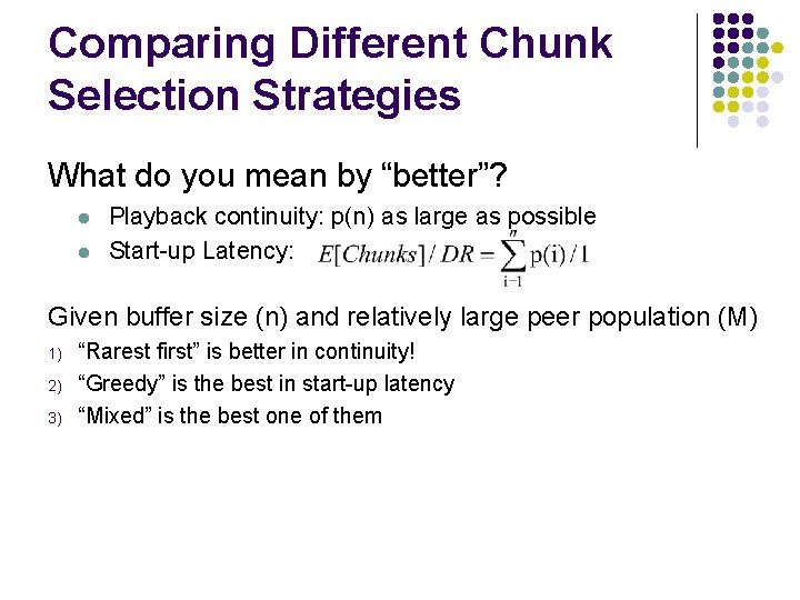
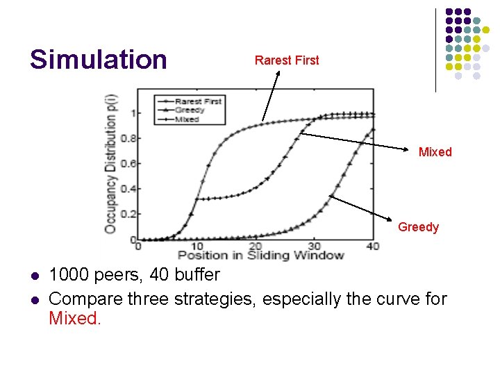
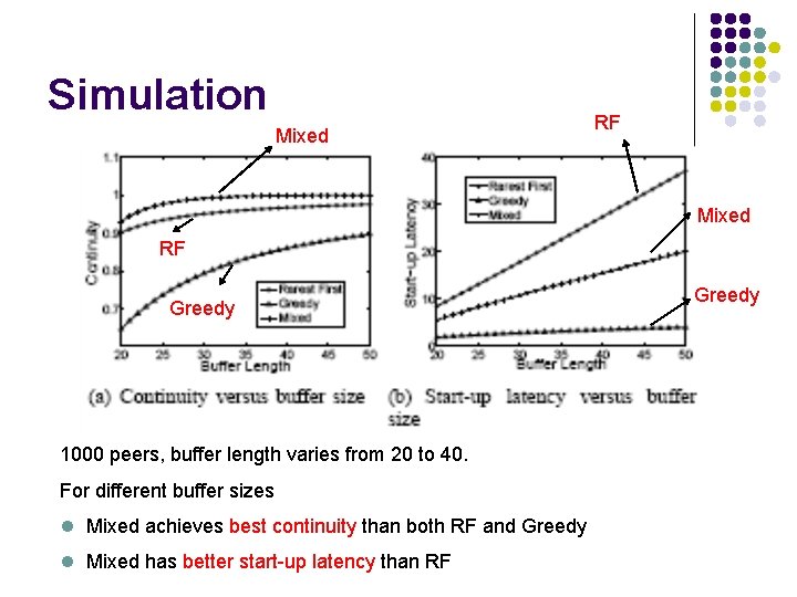
Comparing Different Chunk Selection Strategies What do you mean by “better”? l l Playback continuity: p(n) as large as possible Start-up Latency: Given buffer size (n) and relatively large peer population (M) 1) 2) 3) “Rarest first” is better in continuity! “Greedy” is the best in start-up latency “Mixed” is the best one of them

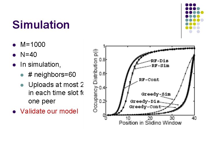
Simulation l l M=1000 N=40 In simulation, l # neighbors=60 l Uploads at most 2 in each time slot for one peer Validate our model

Simulation Rarest First Mixed Greedy l l 1000 peers, 40 buffer Compare three strategies, especially the curve for Mixed.

Simulation Mixed RF Greedy 1000 peers, buffer length varies from 20 to 40. For different buffer sizes l Mixed achieves best continuity than both RF and Greedy l Mixed has better start-up latency than RF Greedy

Simulation RF Greedy l l Greedy RF For (a), there are 40 peers. Greedy is better. For (b), the continuity requirement is fixed at 0. 93. RF is better

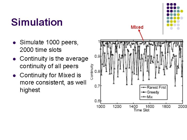
Simulation l l l Simulate 1000 peers, 2000 time slots Continuity is the average continuity of all peers Continuity for Mixed is more consistent, as well highest Mixed

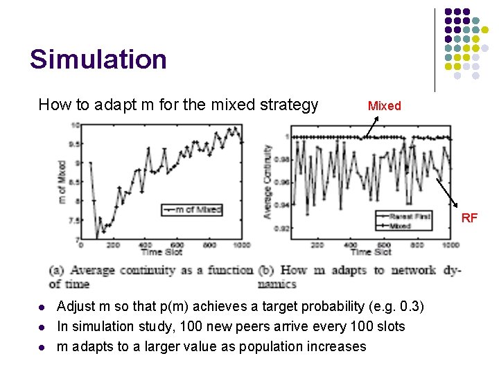
Simulation How to adapt m for the mixed strategy Mixed RF l l l Adjust m so that p(m) achieves a target probability (e. g. 0. 3) In simulation study, 100 new peers arrive every 100 slots m adapts to a larger value as population increases

Outline l l Introduction Model & Chunk Selection Strategies Simulation Conclusion

Conclusion l Related work -Coolstreaming, Bi. Tos l Summary work on p 2 p streaming: -There are many designed p 2 p streaming systems, such as PPLive, PPstream -Many measurement papers on these system -Little work on model analysis -Little study on chunk selection strategies l Our Contribution: -Analytical Models on p 2 p streaming system to better understand -Chunk selection strategy study -Mixed strategy is proposed, which is better than RF or Greedy -Trade off between continuity and scalability