A Review of Some Fundamental Mathematical and Statistical

A Review of Some Fundamental Mathematical and Statistical Concepts Un. B Mestrado em Ciências Contábeis Prof. Otávio Medeiros, MSc, Ph. D

Characteristics of probability distributions • Random variable: can take on any value from a given set • Most commonly used distribution: normal or Gaussian • Normal probability density function:

Characteristics of probability distributions • The mean of a random variable is known as its expected value E(y). • Properties of expected values: – E(c) = c c = constant – E(cy) = c E(y) – E(cy + d) = c E(y) + d d = constant – If y and z are independent, E(yz) = E(y) E(z)

Characteristics of probability distributions • The variance of a random variable is var(y). • Properties of var operator: var(c) = 0 –. – If y and z are independent,

Characteristics of probability distributions • The covariance between 2 random variables is cov(y, z). • Properties of cov operator: – If y and z are independent, cov(y, z) = 0 – If c, d, e, and f are constants

Characteristics of probability distributions • If a random sample of size T: y 1, y 2, . . . , yn is drawn from a normally distributed population with mean m and variance s 2, the sample mean is also normally distributed with mean m and variance s 2/T. • Central limit theorem: sampling distribution of the mean of any random sample tends to the normal distribution with mean m as sample size ® ¥

Properties of logarithms • Logs can have any base, but in finance and economics the neperian or natural log is more usual. Its base is the number e = 2, 7128. . • ln(xy) = ln(x) + ln(y) • ln (x/y) = ln(x) – ln(y) • ln(yc) = c ln(y) • ln(1) = 0 • ln(1/y) = ln(1) – ln(y) = – ln(y)

Differential calculus • The effect of the rate of change of one variable on the rate of change of another is measured by the derivative. • If y = f(x) the derivative of y w. r. t x is • dy/dx or f’(x) measures the instantaneous rate of change of y wrt x

Differential calculus • • Rules: The derivative of a constant is zero If y = 10, dy/dx = 0 If y = 3 x + 2, dy/dx = 3 If y = c xn, dy/dx = cnxn-1 E. g. : y = 4 x 3, dy/dx = 12 x 2

Differential calculus • Rules: • The derivative of a sum is equal to the sum of the derivatives of the individual parts: – E. g. If y = f(x)+g(x), dy/dx = f’(x)+g’(x) • The derivative of the log of x is given by 1/x – d(log(x))/dx = 1/x • The derivative of the log of a function: – d(log(f(x)))/dx=f’(x)/f(x) – E. g. d(log(x 3+2 x-1))=(3 x 2+2)/(x 3+2 x-1)

Differential calculus • • Rules: The derivative of ex = ex The derivative of the ef(x)= f’(x)ef(x) If y = f(x 1, x 2, . . . , xn), the differentiation of y wrt only one variable is the partial differentiation: – E. g.

Differential calculus • The maximum or minimum of a function wrt a variable can be found setting the 1 st derivative f’(x) equal to zero. • Second order condition: – If f”(x)>0 minimum – If f”(x)<0 maximum

Matrices A Matrix is a collection or array of numbers Size of a matrix is given by number of rows and columns R x C If a matrix has only one row, it is a row vector If a matrix has only one column, it is a column vector If R = C the matrix is a square matrix

Definitions • Matrix is a rectangular array of real numbers with R rows and C columns. are matrix elements.

Definitions • • Dimension of a matrix: R x C. Matrix 1 is a scalar. Matrix R x 1 is a column vector. Matrix 1 x C is a row vector. If R = C, the matrix is square. Sum of elements of leading diagonal = trace. Diagonal matrix : square matrix with all elements off the leading diagonal equal to zero. • Identity matrix: diagonal matrix with all elements in the leading diagonal equal to one. • Zero matrix: all elements are zero.

Definitions • Rank of a matrix: is given by the maximum number of linearly independent rows or columns contained in the matrix, e. g. :

Matrix Operations • Equality: A = B if and only if A and B have the same size and aij = bij " i, j. • Addition of matrices: A+B= C if and only if A and B have the same size and aij + bij = cij " i, j.

Matrix operations • Multiplication of a scalar by a matrix: k. A = k. [aij], i. e. every element of the matrix is multiplied by the scalar.

Matrix operations • Multiplication of matrices: if A is m x n and B is n x p, then the product of the 2 matrices is A. B = C, where C is a m x p matrix with elements: • Example: Note: A. B ¹ B. A

Transpose of a matrix • matrix transpose: if A is m x n, then the transpose of A is n x m, i. e. :

Properties of transpose matrices • (A+B)+C=A+(B+C) • (A. B). C=A(B. C)

Square matrices : • Identity matrix I: Note: A. I = I. A = A, where A has the same size as I.

Square matrices : • Diagonal matrix:

Square matrices: • Scalar matrix = diagonal matrix, when l 1 = l 2 =. . . =ln. • Zero matrix: A + 0 = A; A x 0 = 0.

• Trace: If A is m x n and B is n x m, then AB and BA are square matrices and tr(AB) = tr (BA)

Determinants • matrix 2 x 2:

Determinants • matrix 3 x 3:

Determinants • Matrix 3 x 3: Kramer’s rule

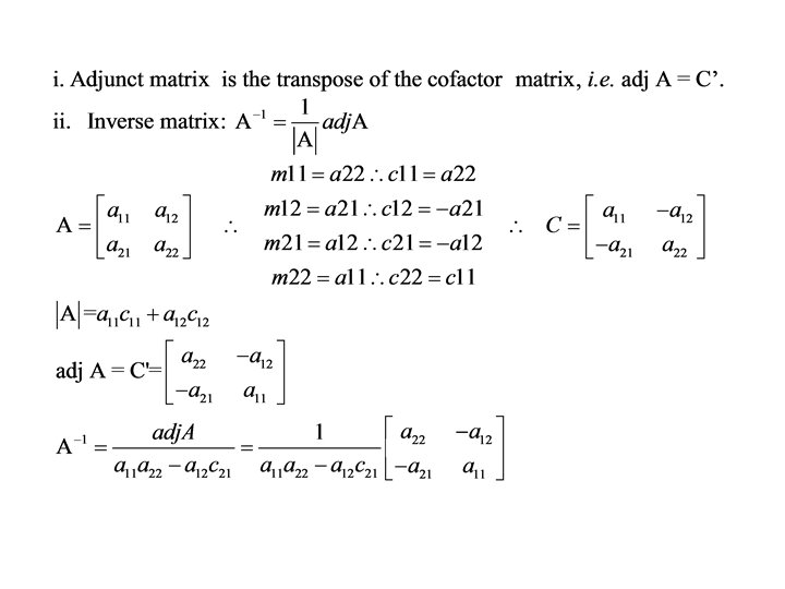
Inverse matrix • The inverse of a square matrix A, named A-1, is the matrix which pre or post multiplied by A gives the identity matrix. • B = A-1 if and only if BA = AB = I • Matrix A has an inverse if and only if det A ¹ 0 (i. e. A is non singular). • (A. B)-1 = B-1. A-1 • (A-1)’=(A’)-1 if A é symmetrical and non singular, then A-1 is symmetrical. • If det A ¹ 0 and A is a square matrix of size n, then A has rank n.

Steps for finding an inverse matrix • Calculation of the determinant: Kramer’s rule or cofactor matrix. • Minor of the element aij is the determinant of the submatrix obtained after exclusion of the i-th row and j-th column. • Cofactor is the minor multiplied by (-1)i+j,

Steps for finding an inverse matrix • Laplace expansion: take any row or column and get the determinant by multiplying the products of each element of row or columns by its respective cofactor. • Cofactor matrix: matrix where each element is substituted by its cofactor.

Example 2 x 2 matrix :

Example • 3 x 3 matrix :

The eigenvalues of a matrix • Let P be a p x p square matrix and let c denote a p x 1 non-zero vector, and let l denote a set of scalars. l is called a characteristic root of the matrix P if it is possible to write: Pc = l. Ipc where Ip is an identity matrix, and hence • (P – l. Ip) c = 0

The eigenvalues of a matrix • Since c ¹ 0 the matrix (P – l. Ip) must be singular (zero determinant) ôP – l. Ipô = 0

The eigenvalues of a matrix • Example: • • Characteristic roots = eigenvalues The sum of eigenvalues = trace of the matrix The product of the eigenvalues = determinant The number of non-zero eigenvalues = rank