A QuickLook DesignofExperiments DOE Orientation Carol Ventresca Carol

A Quick-Look Design-of-Experiments (DOE) Orientation Carol Ventresca Carol @Syn. Genics. com John C. Sparks John@Syn. Genics. com © 2008 Syn. Genics Corporation. All rights reserved.

Presentation Topics u Introductory Experiments with a Black Box Ø Using One-Factor-at-a-Time Methodology Ø Using an Orthogonal Array via a “Designed Experiment” u What Exactly is DOE? Ø History Ø When Applicable u The Classic “Dial Problem” u Air Force Example: Vane Cleaning Experiment u Summary and Resources © 2008 Syn. Genics Corporation. All rights reserved. 2

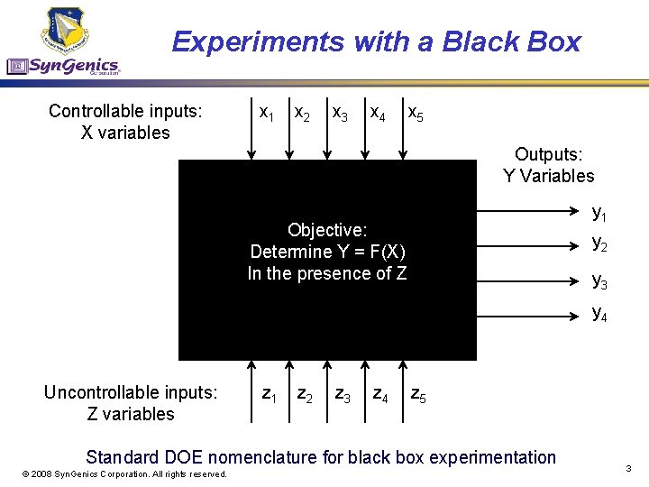
Experiments with a Black Box Controllable inputs: X variables x 1 x 2 x 3 x 4 x 5 Outputs: Y Variables y 1 Objective: Determine Y = F(X) In the presence of Z y 2 y 3 y 4 Uncontrollable inputs: Z variables z 1 z 2 z 3 z 4 z 5 Standard DOE nomenclature for black box experimentation © 2008 Syn. Genics Corporation. All rights reserved. 3

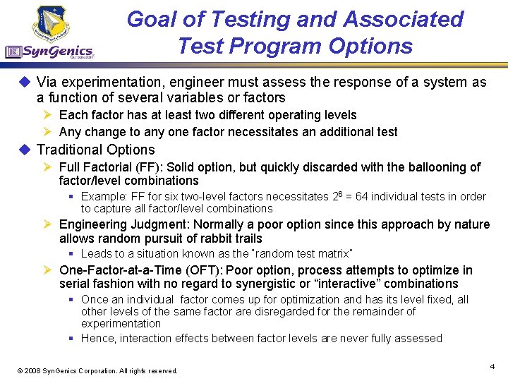
Goal of Testing and Associated Test Program Options u Via experimentation, engineer must assess the response of a system as a function of several variables or factors Ø Each factor has at least two different operating levels Ø Any change to any one factor necessitates an additional test u Traditional Options Ø Full Factorial (FF): Solid option, but quickly discarded with the ballooning of factor/level combinations § Example: FF for six two-level factors necessitates 26 = 64 individual tests in order to capture all factor/level combinations Ø Engineering Judgment: Normally a poor option since this approach by nature allows random pursuit of rabbit trails § Leads to a situation known as the “random test matrix” Ø One-Factor-at-a-Time (OFT): Poor option, process attempts to optimize in serial fashion with no regard to synergistic or “interactive” combinations § Once an individual factor comes up for optimization and has its level fixed, all other levels of the same factor are disregarded for the remainder of experimentation § Hence, interaction effects between factor levels are never fully assessed © 2008 Syn. Genics Corporation. All rights reserved. 4

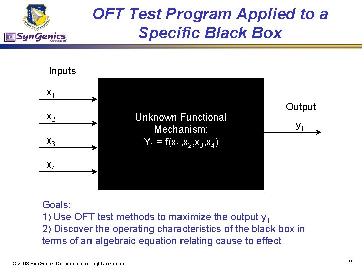
OFT Test Program Applied to a Specific Black Box Inputs x 1 x 2 x 3 Unknown Functional Mechanism: Y 1 = f(x 1, x 2, x 3, x 4) Output y 1 x 4 Goals: 1) Use OFT test methods to maximize the output y 1 2) Discover the operating characteristics of the black box in terms of an algebraic equation relating cause to effect © 2008 Syn. Genics Corporation. All rights reserved. 5

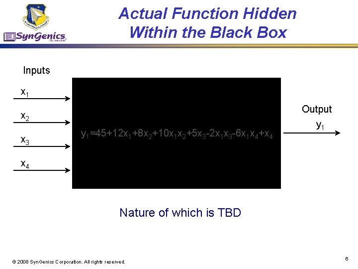
Actual Function Hidden Within the Black Box Inputs x 1 Output x 2 x 3 y 1=45+12 x 1+8 x 2+10 x 1 x 2+5 x 3 -2 x 1 x 3 -6 x 1 x 4+x 4 y 1 x 4 Nature of which is TBD © 2008 Syn. Genics Corporation. All rights reserved. 6

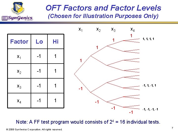
OFT Factors and Factor Levels (Chosen for Illustration Purposes Only) x 1 Factor Lo x 2 x 3 1 Hi x 4 1 1, 1, 1, 1 1 x 1 -1 1 x 2 -1 1 x 3 -1 1 x 4 -1 1 1 -1, 1, -1, 1 -1 -1 -1, -1, -1 Note: A FF test program would consists of 24 = 16 individual tests. © 2008 Syn. Genics Corporation. All rights reserved. 7

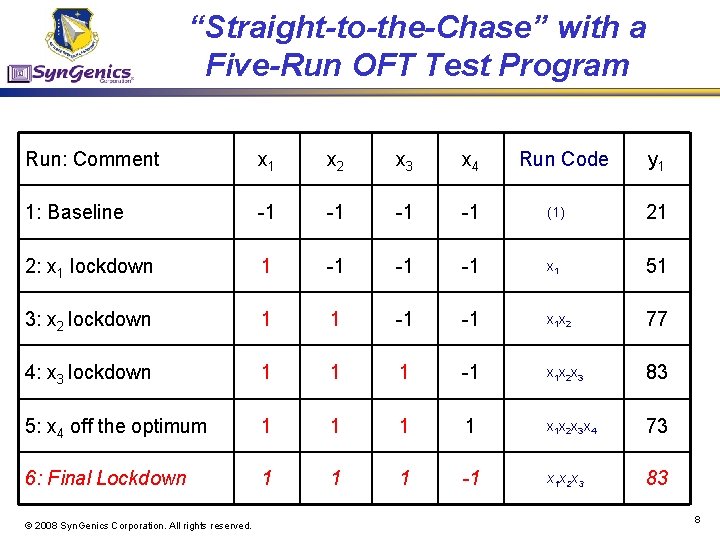
“Straight-to-the-Chase” with a Five-Run OFT Test Program Run: Comment x 1 x 2 x 3 x 4 1: Baseline -1 -1 (1) 21 2: x 1 lockdown 1 -1 -1 -1 x 1 51 3: x 2 lockdown 1 1 -1 -1 x 1 x 2 77 4: x 3 lockdown 1 1 1 -1 x 1 x 2 x 3 83 5: x 4 off the optimum 1 1 x 1 x 2 x 3 x 4 73 6: Final Lockdown 1 1 1 -1 x 1 x 2 x 3 83 © 2008 Syn. Genics Corporation. All rights reserved. Run Code y 1 8

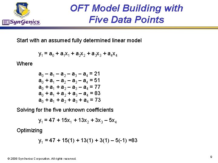
OFT Model Building with Five Data Points Start with an assumed fully determined linear model y 1 = a 0 + a 1 x 1 + a 2 x 2 + a 3 x 3 + a 4 x 4 Where a 0 – a 1 – a 2 – a 3 – a 4 = 21 a 0 + a 1 – a 2 – a 3 – a 4 = 51 a 0 + a 1 + a 2 – a 3 – a 4 = 77 a 0 + a 1 + a 2 + a 3 – a 4 = 83 a 0 + a 1 + a 2 + a 3 + a 4 = 73 Solving for the five unknown coefficients y 1 = 47 + 15 x 1 + 13 x 2 + 3 x 3 – 5 x 4 Optimizing y 1 = 47 + 15(1) + 13(1) + 3(1) – 5(-1) =83 © 2008 Syn. Genics Corporation. All rights reserved. 9

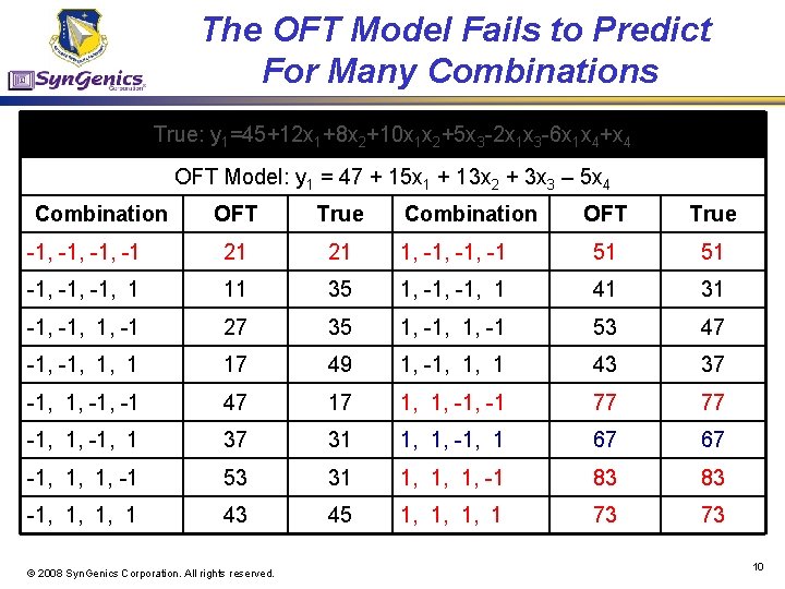
The OFT Model Fails to Predict For Many Combinations True: y 1=45+12 x 1+8 x 2+10 x 1 x 2+5 x 3 -2 x 1 x 3 -6 x 1 x 4+x 4 OFT Model: y 1 = 47 + 15 x 1 + 13 x 2 + 3 x 3 – 5 x 4 Combination OFT True -1, -1, -1 21 21 -1, -1, 1 11 -1, 1, -1 OFT True 1, -1, -1 51 51 35 1, -1, 1 41 31 27 35 1, -1, 1, -1 53 47 -1, 1, 1 17 49 1, -1, 1, 1 43 37 -1, 1, -1 47 17 1, 1, -1 77 77 -1, 1, -1, 1 37 31 1, 1, -1, 1 67 67 -1, 1, 1, -1 53 31 1, 1, 1, -1 83 83 -1, 1, 1, 1 43 45 1, 1, 1, 1 73 73 © 2008 Syn. Genics Corporation. All rights reserved. Combination 10

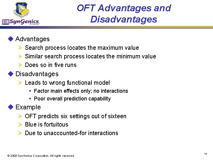
OFT Advantages and Disadvantages u Advantages Ø Search process locates the maximum value Ø Similar search process locates the minimum value Ø Does so in five runs u Disadvantages Ø Leads to wrong functional model § Factor main effects only; no interactions § Poor overall prediction capability u Example Ø OFT predicts six settings out of sixteen Ø Blue is fortuitous Ø Due to unaccounted-for interactions © 2008 Syn. Genics Corporation. All rights reserved. 11

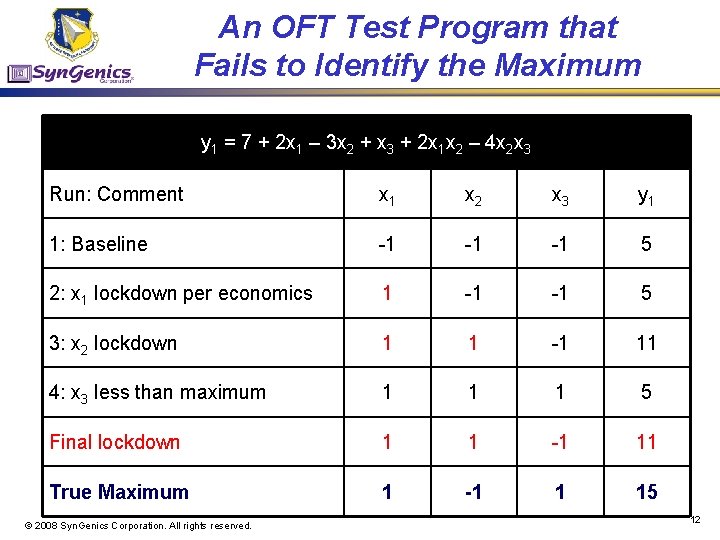
An OFT Test Program that Fails to Identify the Maximum y 1 = 7 + 2 x 1 – 3 x 2 + x 3 + 2 x 1 x 2 – 4 x 2 x 3 Run: Comment x 1 x 2 x 3 y 1 1: Baseline -1 -1 -1 5 2: x 1 lockdown per economics 1 -1 -1 5 3: x 2 lockdown 1 1 -1 11 4: x 3 less than maximum 1 1 1 5 Final lockdown 1 1 -1 11 True Maximum 1 -1 1 15 © 2008 Syn. Genics Corporation. All rights reserved. 12

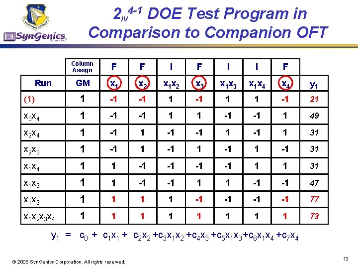
2 IV 4 -1 DOE Test Program in Comparison to Companion OFT Column Assign F F I I F GM x 1 x 2 x 3 x 1 x 4 y 1 (1) 1 -1 -1 1 1 -1 21 x 3 x 4 1 -1 -1 1 49 x 2 x 4 1 -1 -1 1 31 x 2 x 3 1 -1 31 x 1 x 4 1 1 -1 -1 1 1 31 x 1 x 3 1 1 -1 -1 47 x 1 x 2 1 1 -1 -1 77 x 1 x 2 x 3 x 4 1 1 1 1 73 Run y 1 = c 0 + c 1 x 1 + c 2 x 2 +c 3 x 1 x 2 +c 4 x 3 +c 5 x 1 x 3+c 6 x 1 x 4 +c 7 x 4 © 2008 Syn. Genics Corporation. All rights reserved. 13

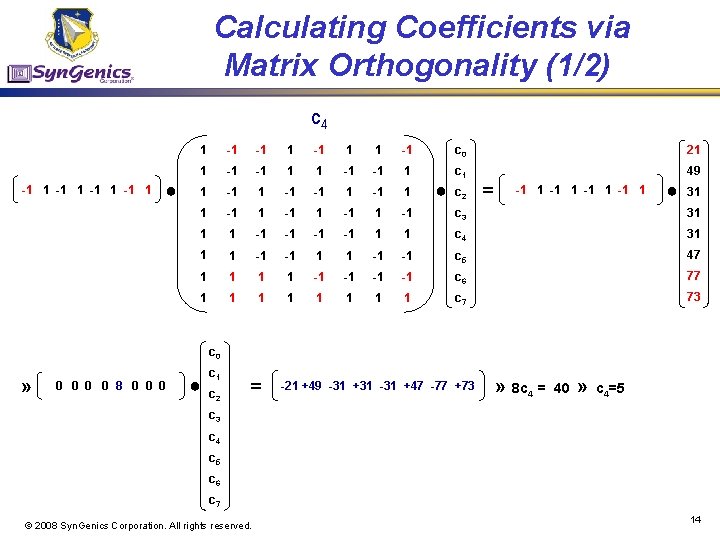
Calculating Coefficients via Matrix Orthogonality (1/2) c 4 -1 1 ● 1 -1 -1 1 1 -1 c 0 21 1 -1 -1 1 c 1 49 1 -1 -1 1 -1 c 3 31 1 1 -1 -1 1 1 c 4 31 1 1 -1 -1 c 5 47 1 1 -1 -1 c 6 77 1 1 1 1 c 7 73 ● c 2 = -1 1 ● 31 c 0 » 0 0 8 0 0 0 ● c 1 c 2 = -21 +49 -31 +31 -31 +47 -77 +73 » 8 c 4 = 40 » c 4=5 c 3 c 4 c 5 c 6 c 7 © 2008 Syn. Genics Corporation. All rights reserved. 14

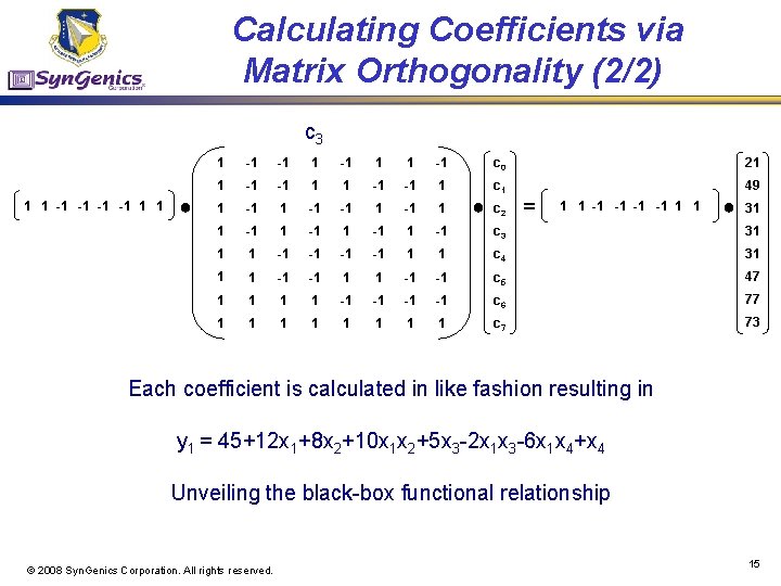
Calculating Coefficients via Matrix Orthogonality (2/2) c 3 1 1 -1 -1 1 1 ● 1 -1 -1 1 1 -1 c 0 21 1 -1 -1 1 c 1 49 1 -1 -1 1 -1 c 3 31 1 1 -1 -1 1 1 c 4 31 1 1 -1 -1 c 5 47 1 1 -1 -1 c 6 77 1 1 1 1 c 7 73 ● c 2 = 1 1 -1 -1 1 1 ● 31 Each coefficient is calculated in like fashion resulting in y 1 = 45+12 x 1+8 x 2+10 x 1 x 2+5 x 3 -2 x 1 x 3 -6 x 1 x 4+x 4 Unveiling the black-box functional relationship © 2008 Syn. Genics Corporation. All rights reserved. 15

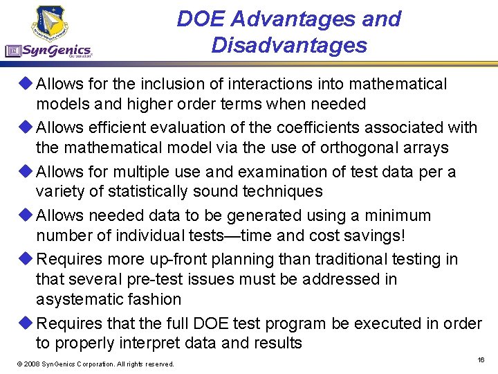
DOE Advantages and Disadvantages u Allows for the inclusion of interactions into mathematical models and higher order terms when needed u Allows efficient evaluation of the coefficients associated with the mathematical model via the use of orthogonal arrays u Allows for multiple use and examination of test data per a variety of statistically sound techniques u Allows needed data to be generated using a minimum number of individual tests—time and cost savings! u Requires more up-front planning than traditional testing in that several pre-test issues must be addressed in asystematic fashion u Requires that the full DOE test program be executed in order to properly interpret data and results © 2008 Syn. Genics Corporation. All rights reserved. 16

What Exactly is DOE? u DOE is one of the core “Six-Sigma” methodologies Ø Statistically selects “axiomatic points” in the design space Ø Selection enables maximum information return on investment made Ø Used to systematically analyze the nature and cause of variation by means of controlled testing (as opposed to examining available data) Ø Cause is linked to effect by establishing through experimentation the coefficients for pre-determined “best-fit” models § Linear models: two-level experiments § Piece-wise linear models: multi-level “orthogonal type” experiments § Non-linear (general second-order quadratic model): response surface methods u Test programs built upon sound DOE principles are Ø Significantly compressed and extremely efficient Ø Produce high-quality and reusable data © 2008 Syn. Genics Corporation. All rights reserved. 17

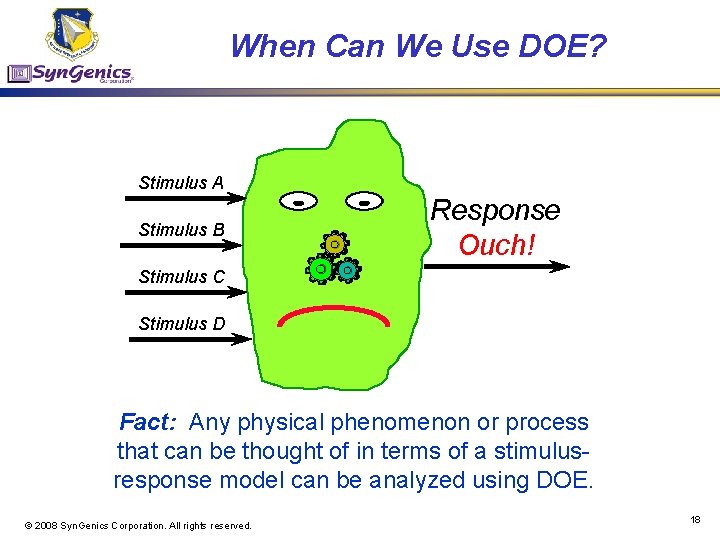
When Can We Use DOE? Stimulus A Stimulus B Response Ouch! Stimulus C Stimulus D Fact: Any physical phenomenon or process that can be thought of in terms of a stimulusresponse model can be analyzed using DOE. © 2008 Syn. Genics Corporation. All rights reserved. 18

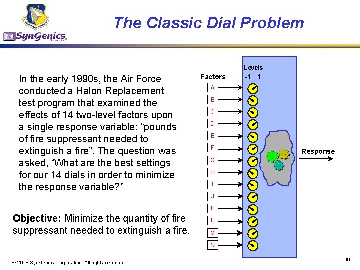
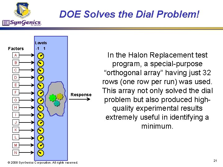
The Classic Dial Problem Levels In the early 1990 s, the Air Force conducted a Halon Replacement test program that examined the effects of 14 two-level factors upon a single response variable: “pounds of fire suppressant needed to extinguish a fire”. The question was asked, “What are the best settings for our 14 dials in order to minimize the response variable? ” Factors -1 1 A B C D E F Response G H I J K Objective: Minimize the quantity of fire suppressant needed to extinguish a fire. L M N © 2008 Syn. Genics Corporation. All rights reserved. 19

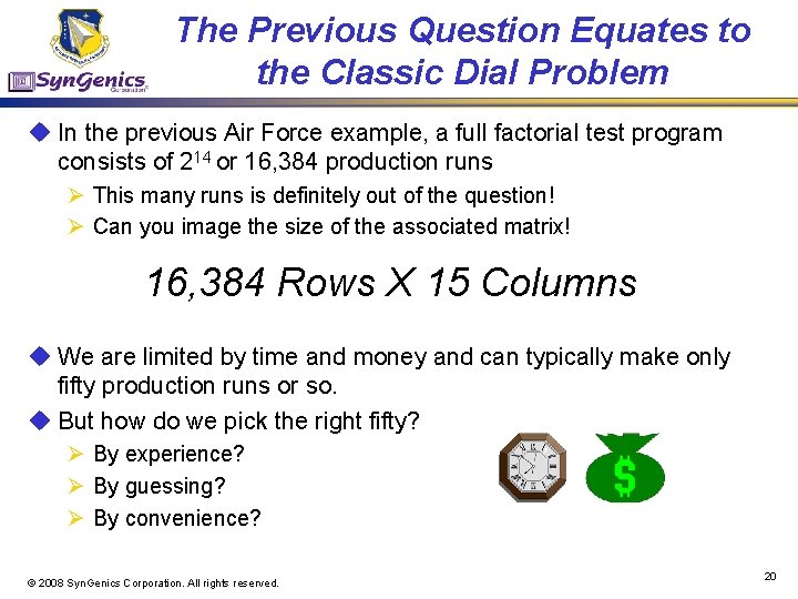
The Previous Question Equates to the Classic Dial Problem u In the previous Air Force example, a full factorial test program consists of 214 or 16, 384 production runs Ø This many runs is definitely out of the question! Ø Can you image the size of the associated matrix! 16, 384 Rows X 15 Columns u We are limited by time and money and can typically make only fifty production runs or so. u But how do we pick the right fifty? Ø By experience? Ø By guessing? Ø By convenience? © 2008 Syn. Genics Corporation. All rights reserved. 20

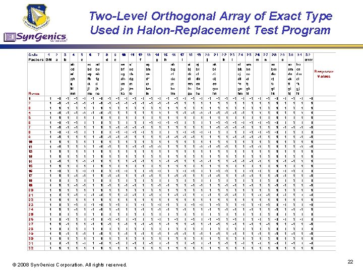
DOE Solves the Dial Problem! Levels Factors -1 1 A B C D E F Response G H I J K In the Halon Replacement test program, a special-purpose “orthogonal array” having just 32 rows (one row per run) was used. This array not only solved the dial problem but also produced highquality experimental results extremely useful in identifying a minimum. L M N © 2008 Syn. Genics Corporation. All rights reserved. 21

Two-Level Orthogonal Array of Exact Type Used in Halon-Replacement Test Program © 2008 Syn. Genics Corporation. All rights reserved. 22

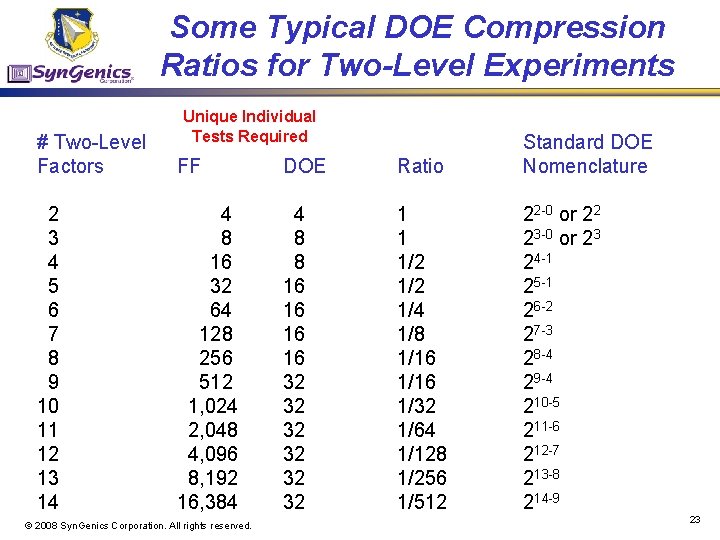
Some Typical DOE Compression Ratios for Two-Level Experiments Unique Individual Tests Required # Two-Level Factors FF DOE Ratio Standard DOE Nomenclature 2 3 4 5 6 7 8 9 10 11 12 13 14 4 8 16 32 64 128 256 512 1, 024 2, 048 4, 096 8, 192 16, 384 4 8 8 16 16 32 32 32 1 1 1/2 1/4 1/8 1/16 1/32 1/64 1/128 1/256 1/512 22 -0 or 22 23 -0 or 23 24 -1 25 -1 26 -2 27 -3 28 -4 29 -4 210 -5 211 -6 212 -7 213 -8 214 -9 © 2008 Syn. Genics Corporation. All rights reserved. 23

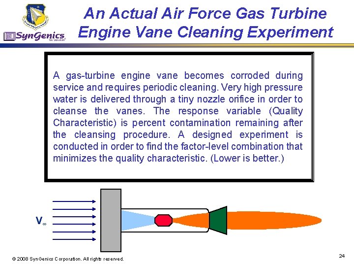
An Actual Air Force Gas Turbine Engine Vane Cleaning Experiment A gas-turbine engine vane becomes corroded during service and requires periodic cleaning. Very high pressure water is delivered through a tiny nozzle orifice in order to cleanse the vanes. The response variable (Quality Characteristic) is percent contamination remaining after the cleansing procedure. A designed experiment is conducted in order to find the factor-level combination that minimizes the quality characteristic. (Lower is better. ) V∞ © 2008 Syn. Genics Corporation. All rights reserved. 24

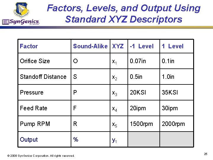
Factors, Levels, and Output Using Standard XYZ Descriptors Factor Sound-Alike XYZ -1 Level Orifice Size O x 1 0. 07 in 0. 1 in Standoff Distance S x 2 0. 5 in 1. 0 in Pressure P x 3 20 KSI 35 KSI Feed Rate F x 4 20 ipm 30 ipm Pump RPM R x 5 1500 rpm 2000 rpm Output % y 1 © 2008 Syn. Genics Corporation. All rights reserved. 25

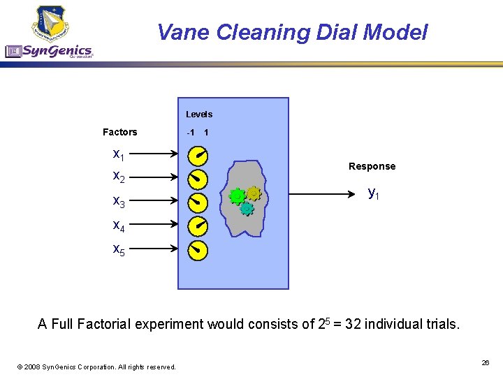
Vane Cleaning Dial Model Levels Factors x 1 x 2 x 3 -1 1 Response y 1 x 4 x 5 A Full Factorial experiment would consists of 25 = 32 individual trials. © 2008 Syn. Genics Corporation. All rights reserved. 26

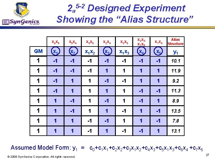
2 III 5 -2 Designed Experiment Showing the “Alias Structure” x 4 x 5 x 3 x 4 x 3 x 5 x 2 x 4 x 2 x 5 x 2 x 3 x 1 x 5 x 1 x 4 Alias Structure GM x 1 x 2 x 3 x 1 x 3 x 4 x 5 y 1 1 -1 -1 10. 1 1 -1 -1 -1 1 1 11. 9 1 -1 1 1 -1 -1 1 1 9. 2 1 -1 1 1 -1 -1 11. 3 1 1 -1 1 8. 9 1 1 -1 13. 5 1 1 1 -1 -1 1 1 -1 7. 8 1 1 1 -1 -1 1 13. 1 Assumed Model Form: y 1 = c 0+c 1 x 1+c 2 x 2+c 3 x 1 x 2+c 4 x 3+c 5 x 1 x 3+c 6 x 4 +c 7 x 5 © 2008 Syn. Genics Corporation. All rights reserved. 27

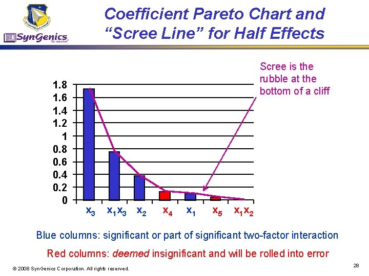
Coefficient Pareto Chart and “Scree Line” for Half Effects 1. 8 1. 6 1. 4 1. 2 1 0. 8 0. 6 0. 4 0. 2 0 Scree is the rubble at the bottom of a cliff x 3 x 1 x 3 x 2 x 4 x 1 x 5 x 1 x 2 Blue columns: significant or part of significant two-factor interaction Red columns: deemed insignificant and will be rolled into error © 2008 Syn. Genics Corporation. All rights reserved. 28

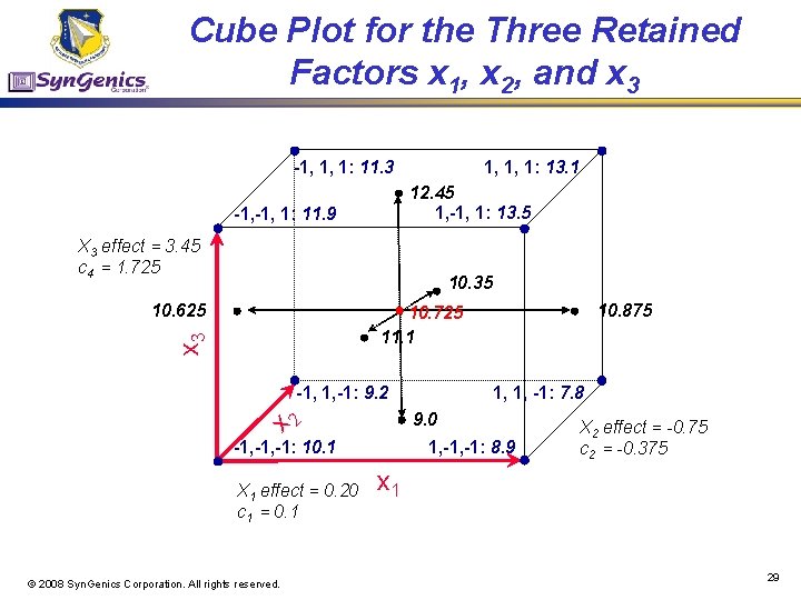
Cube Plot for the Three Retained Factors x 1, x 2, and x 3 -1, 1, 1: 11. 3 1, 1, 1: 13. 1 12. 45 1, -1, 1: 13. 5 -1, 1: 11. 9 X 3 effect = 3. 45 c 4 = 1. 725 10. 35 10. 625 10. 875 x 3 10. 725 11. 1 -1, 1, -1: 9. 2 x 2 9. 0 -1, -1: 10. 1 X 1 effect = 0. 20 c 1 = 0. 1 © 2008 Syn. Genics Corporation. All rights reserved. 1, 1, -1: 7. 8 1, -1: 8. 9 X 2 effect = -0. 75 c 2 = -0. 375 x 1 29

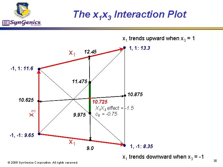
The x 1 x 3 Interaction Plot x 1 trends upward when x 3 = 1 x 1 12. 45 1, 1: 13. 3 -1, 1: 11. 6 11. 475 10. 875 x 3 10. 625 -1, -1: 9. 65 9. 975 x 1 10. 725 X 1 X 3 effect = -1. 5 c 5 = -0. 75 9. 0 1, -1: 8. 35 x 1 trends downward when x 3 = -1 © 2008 Syn. Genics Corporation. All rights reserved. 30

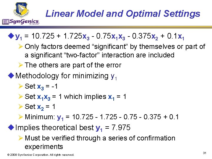
Linear Model and Optimal Settings u y 1 = 10. 725 + 1. 725 x 3 - 0. 75 x 1 x 3 - 0. 375 x 2 + 0. 1 x 1 Ø Only factors deemed “significant” by themselves or part of a significant “two-factor” interaction are included Ø The others are part of the error u Methodology for minimizing y 1 Ø Set x 3 = -1 Ø Set x 1 x 3 = 1 which implies x 1 = 1 Ø Set x 2 = 1 Ø Minimum: y 1 = 10. 725 - 1. 725 - 0. 75 - 0. 375 + 0. 1 u Implies theoretical best y 1 = 7. 975 Ø Must be verified through a series of confirmation experiments © 2008 Syn. Genics Corporation. All rights reserved. 31

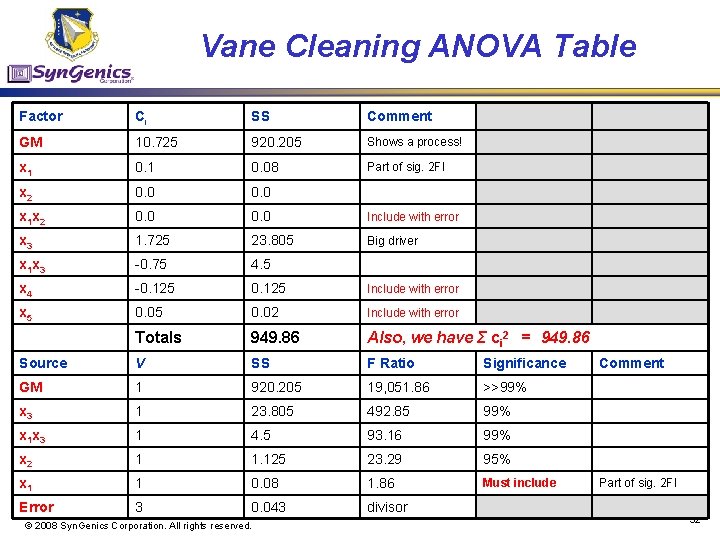
Vane Cleaning ANOVA Table Factor Ci SS Comment GM 10. 725 920. 205 Shows a process! x 1 0. 08 Part of sig. 2 FI x 2 0. 0 x 1 x 2 0. 0 Include with error x 3 1. 725 23. 805 Big driver x 1 x 3 -0. 75 4. 5 x 4 -0. 125 Include with error x 5 0. 02 Include with error Totals 949. 86 Also, we have Σ ci 2 = 949. 86 Source V SS F Ratio Significance GM 1 920. 205 19, 051. 86 >>99% x 3 1 23. 805 492. 85 99% x 1 x 3 1 4. 5 93. 16 99% x 2 1 1. 125 23. 29 95% x 1 1 0. 08 1. 86 Must include Error 3 0. 043 divisor © 2008 Syn. Genics Corporation. All rights reserved. Comment Part of sig. 2 FI 32

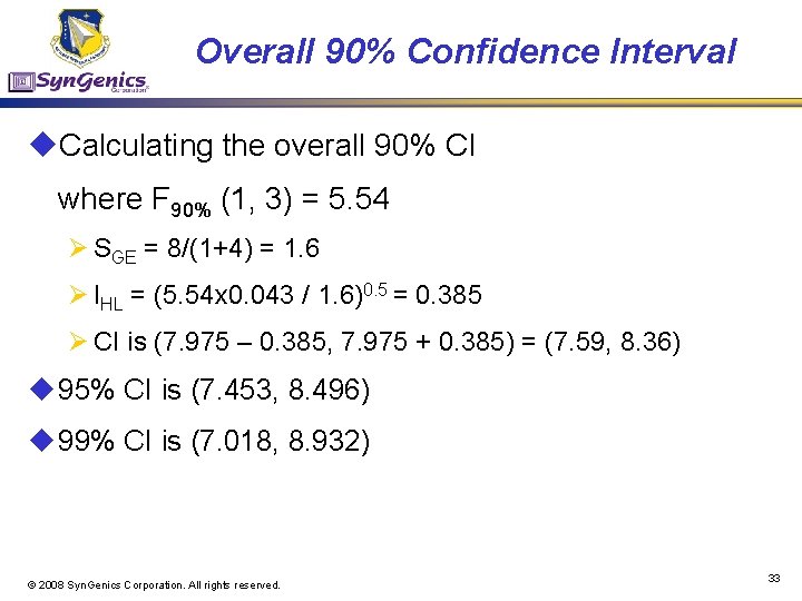
Overall 90% Confidence Interval u. Calculating the overall 90% CI where F 90% (1, 3) = 5. 54 Ø SGE = 8/(1+4) = 1. 6 Ø IHL = (5. 54 x 0. 043 / 1. 6)0. 5 = 0. 385 Ø CI is (7. 975 – 0. 385, 7. 975 + 0. 385) = (7. 59, 8. 36) u 95% CI is (7. 453, 8. 496) u 99% CI is (7. 018, 8. 932) © 2008 Syn. Genics Corporation. All rights reserved. 33

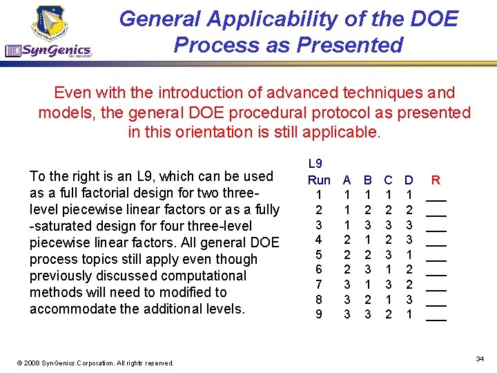
General Applicability of the DOE Process as Presented Even with the introduction of advanced techniques and models, the general DOE procedural protocol as presented in this orientation is still applicable. To the right is an L 9, which can be used as a full factorial design for two threelevel piecewise linear factors or as a fully -saturated design for four three-level piecewise linear factors. All general DOE process topics still apply even though previously discussed computational methods will need to modified to accommodate the additional levels. © 2008 Syn. Genics Corporation. All rights reserved. L 9 Run A 1 1 2 1 3 1 4 2 5 2 6 2 7 3 8 3 9 3 B C D R 1 1 1 ___ 2 2 2 ___ 3 3 3 ___ 1 2 3 ___ 2 3 1 ___ 3 1 2 ___ 1 3 2 ___ 2 1 3 ___ 3 2 1 ___ 34

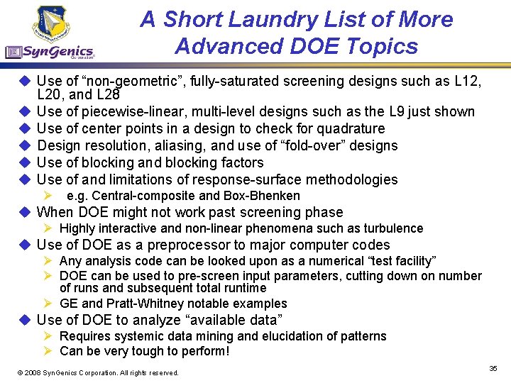
A Short Laundry List of More Advanced DOE Topics u Use of “non-geometric”, fully-saturated screening designs such as L 12, L 20, and L 28 u Use of piecewise-linear, multi-level designs such as the L 9 just shown u Use of center points in a design to check for quadrature u Design resolution, aliasing, and use of “fold-over” designs u Use of blocking and blocking factors u Use of and limitations of response-surface methodologies Ø e. g. Central-composite and Box-Bhenken u When DOE might not work past screening phase Ø Highly interactive and non-linear phenomena such as turbulence u Use of DOE as a preprocessor to major computer codes Ø Any analysis code can be looked upon as a numerical “test facility” Ø DOE can be used to pre-screen input parameters, cutting down on number of runs and subsequent total runtime Ø GE and Pratt-Whitney notable examples u Use of DOE to analyze “available data” Ø Requires systemic data mining and elucidation of patterns Ø Can be very tough to perform! © 2008 Syn. Genics Corporation. All rights reserved. 35

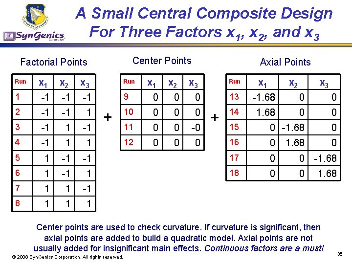
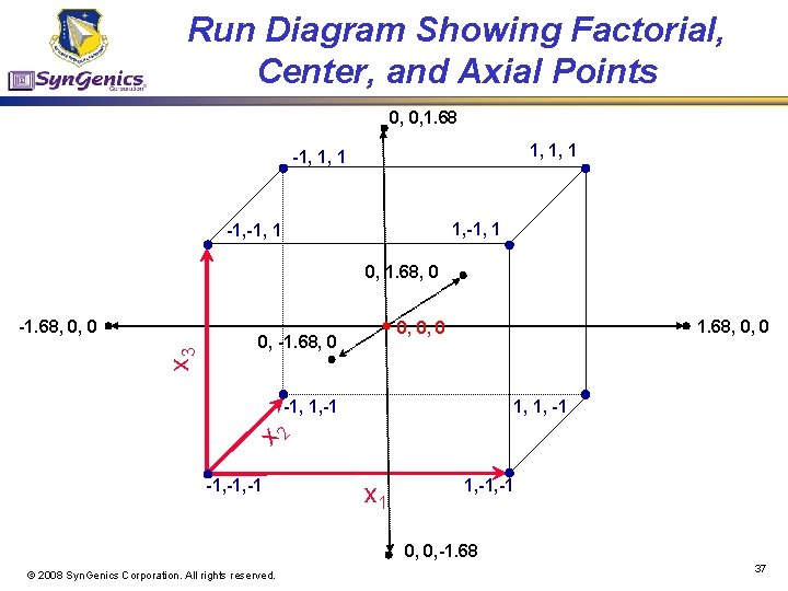
A Small Central Composite Design For Three Factors x 1, x 2, and x 3 Center Points Factorial Points x 1 x 2 x 3 1 -1 -1 -1 2 -1 -1 1 3 -1 1 -1 4 -1 1 1 5 1 -1 6 1 7 8 Run Axial Points x 1 x 2 x 3 9 0 0 11 12 Run x 1 0 13 -1. 68 0 0 14 1. 68 0 0 -0 15 0 -1. 68 0 0 16 0 1. 68 0 -1 17 0 0 -1. 68 -1 1 18 0 0 1. 68 1 1 -1 1 Run + + x 2 x 3 Center points are used to check curvature. If curvature is significant, then axial points are added to build a quadratic model. Axial points are not usually added for insignificant main effects. Continuous factors are a must! © 2008 Syn. Genics Corporation. All rights reserved. 36

Run Diagram Showing Factorial, Center, and Axial Points 0, 0, 1. 68 1, 1, 1 -1, 1, 1 1, -1, 1 0, 1. 68, 0 x 3 -1. 68, 0, 0 0, -1. 68, 0 1, 1, -1 x 2 -1, 1, -1 -1, -1 x 1 1, -1 0, 0, -1. 68 © 2008 Syn. Genics Corporation. All rights reserved. 37

Syn. Genics Two-Day DOE Course Description and Objectives u Course Description Ø Basic introduction to “two-level” DOE that includes § § § The importance of experimental design How to plan and design an experiment The role and use of “orthogonal” arrays How to conduct a statistically designed experiment How to analyze results from a statistically designed experiment Ø Take-away tool box in this course is limited to two-level designs and associated analysis techniques u Course Objectives Ø Be able to plan, execute, and analyze a simple two-level designed experiment Ø Be able to understand assess more complex two-level designed experiments as presented by Air Force contractors Ø Be cognizant of advanced DOE methodologies that go beyond the basic two-level designs © 2008 Syn. Genics Corporation. All rights reserved. 38

© 2008 Syn. Genics Corporation. All rights reserved. 39