A Primer on the Exponential Family of Distributions
A Primer on the Exponential Family of Distributions David Clark & Charles Thayer American Re-Insurance GLM Call Paper - 2004

Agenda • Brief Introduction to GLM • Overview of the Exponential Family • Some Specific Distributions • Suggestions for Insurance Applications 2
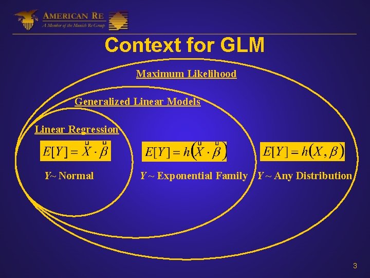
Context for GLM Maximum Likelihood Generalized Linear Models Linear Regression Y~ Normal Y ~ Exponential Family Y ~ Any Distribution 3
Advantages over Linear Regression • Instead of linear combination of covariates, we can use a function of a linear combination of covariates • Response variable stays in original units • Great flexibility in variance structure 4
![Transforming the Response versus Transforming the Covariates Linear Regression E[g(y)] = X· GLM E[y] Transforming the Response versus Transforming the Covariates Linear Regression E[g(y)] = X· GLM E[y]](http://slidetodoc.com/presentation_image_h2/442f53b2372c661a5f8225c75c325dd0/image-5.jpg)
Transforming the Response versus Transforming the Covariates Linear Regression E[g(y)] = X· GLM E[y] = g-1(X· ) Note that if g(y)=ln(y), then Linear Regression cannot handle any points where y 0. 5
Advantages of this Special Case of Maximum Likelihood • Pre-programmed in many software packages • Direct calculation of standard errors of key parameters • Convenient separation of Mean parameter from “nuisance” parameters 6
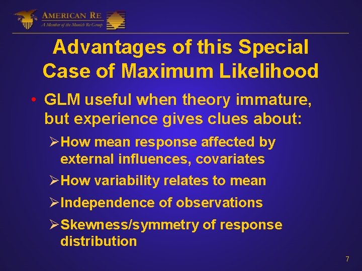
Advantages of this Special Case of Maximum Likelihood • GLM useful when theory immature, but experience gives clues about: ØHow mean response affected by external influences, covariates ØHow variability relates to mean ØIndependence of observations ØSkewness/symmetry of response distribution 7
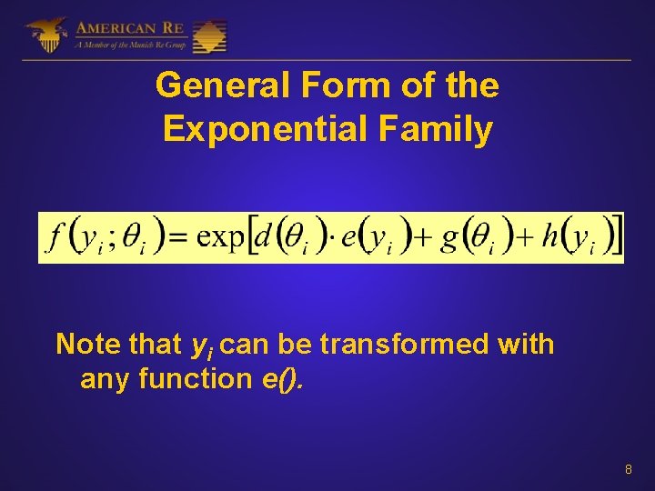
General Form of the Exponential Family Note that yi can be transformed with any function e(). 8
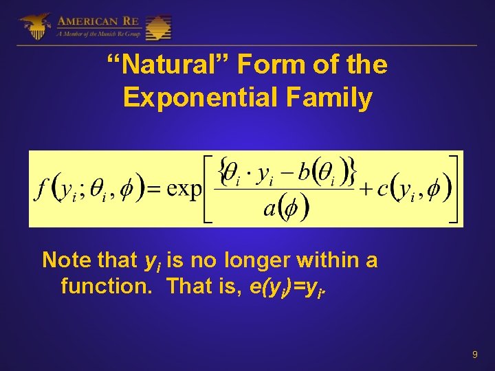
“Natural” Form of the Exponential Family Note that yi is no longer within a function. That is, e(yi)=yi. 9
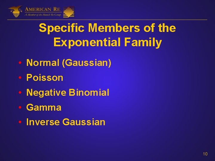
Specific Members of the Exponential Family • Normal (Gaussian) • Poisson • Negative Binomial • Gamma • Inverse Gaussian 10
Some Other Members of the Exponential Family • Natural Form ØBinomial ØLogarithmic ØCompound Poisson/Gamma (Tweedie) • General Form [use ln(y) instead of y] ØLognormal ØSingle Parameter Pareto 11
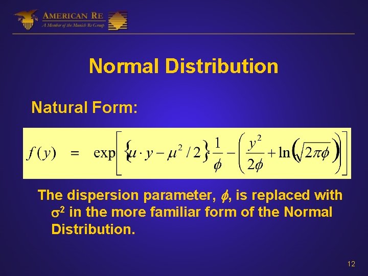
Normal Distribution Natural Form: The dispersion parameter, , is replaced with 2 in the more familiar form of the Normal Distribution. 12
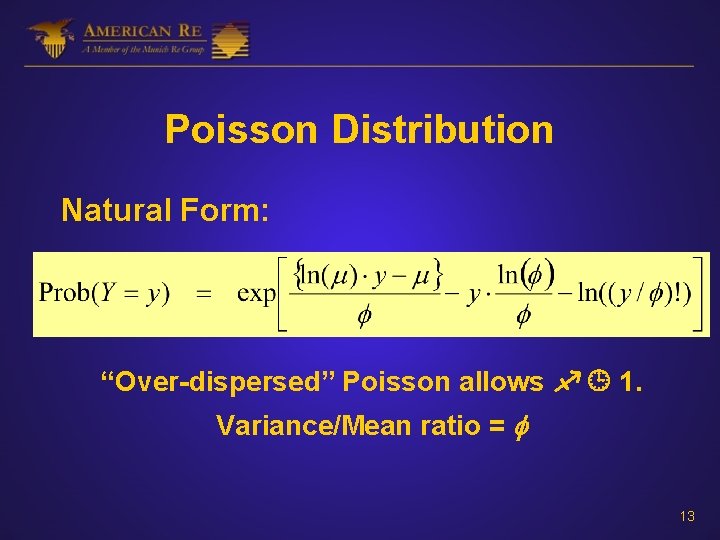
Poisson Distribution Natural Form: “Over-dispersed” Poisson allows 1. Variance/Mean ratio = 13
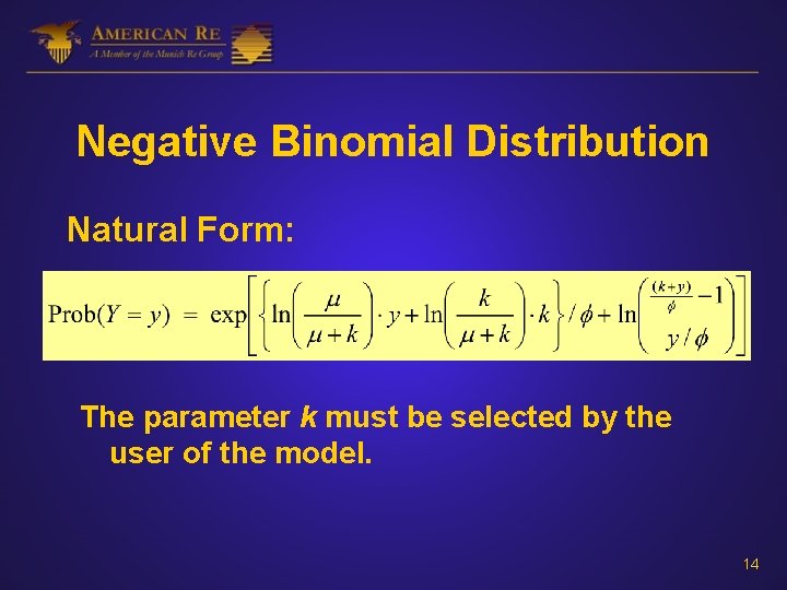
Negative Binomial Distribution Natural Form: The parameter k must be selected by the user of the model. 14
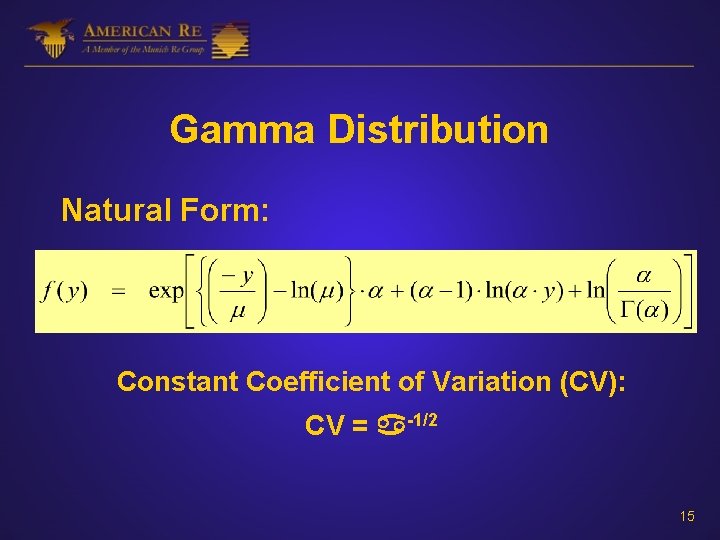
Gamma Distribution Natural Form: Constant Coefficient of Variation (CV): CV = -1/2 15
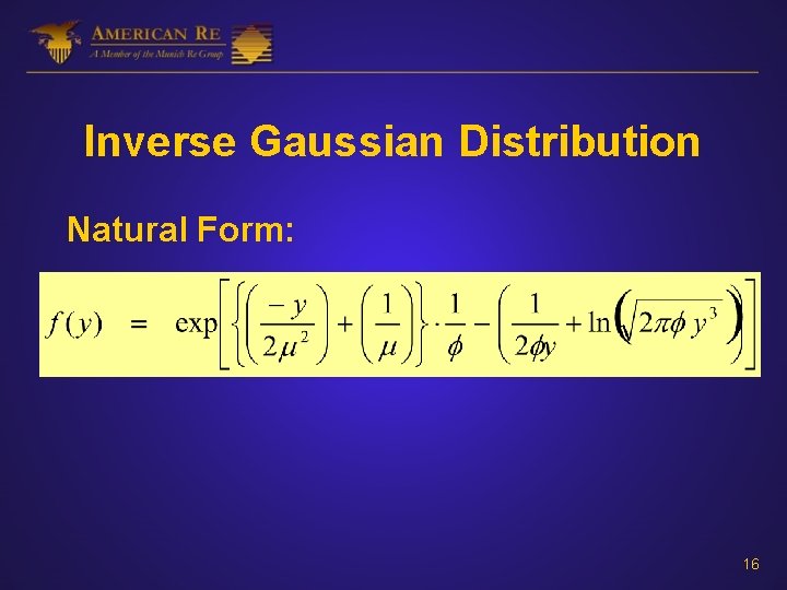
Inverse Gaussian Distribution Natural Form: 16
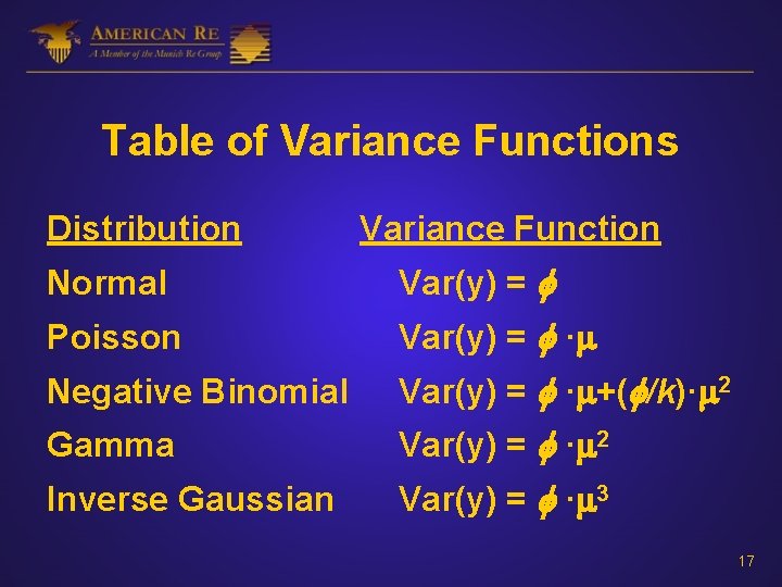
Table of Variance Functions Distribution Variance Function Normal Var(y) = Poisson Var(y) = · Negative Binomial Var(y) = · +( /k)· 2 Gamma Var(y) = · 2 Inverse Gaussian Var(y) = · 3 17
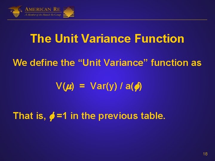
The Unit Variance Function We define the “Unit Variance” function as V( ) = Var(y) / a( ) That is, =1 in the previous table. 18
Uniqueness Property The unit variance function V( ) uniquely identifies its parent distribution type within the natural exponential family. f(y) V( ) 19
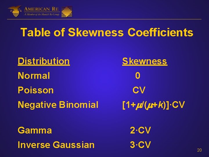
Table of Skewness Coefficients Distribution Skewness Normal 0 Poisson CV Negative Binomial [1+ /( +k)]·CV Gamma 2·CV Inverse Gaussian 3·CV 20
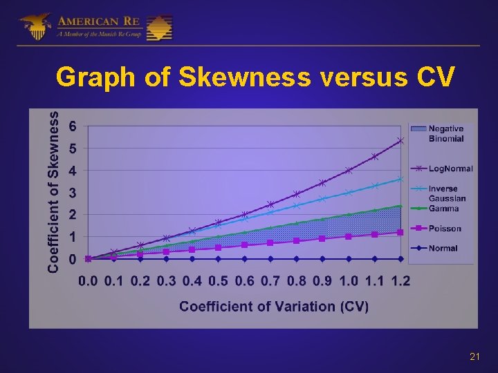
Graph of Skewness versus CV 21

The Big Question: What should the variance function look like for insurance applications? 22
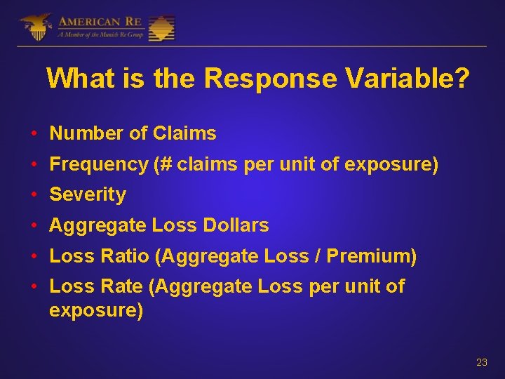
What is the Response Variable? • Number of Claims • Frequency (# claims per unit of exposure) • Severity • Aggregate Loss Dollars • Loss Ratio (Aggregate Loss / Premium) • Loss Rate (Aggregate Loss per unit of exposure) 23
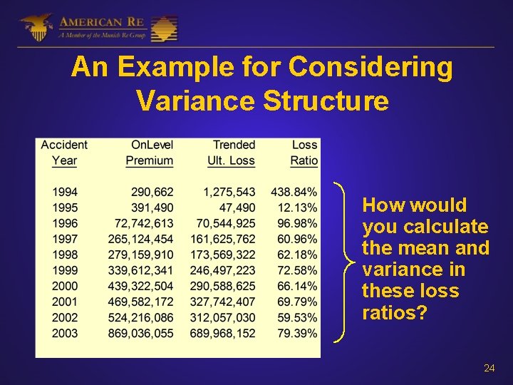
An Example for Considering Variance Structure How would you calculate the mean and variance in these loss ratios? 24
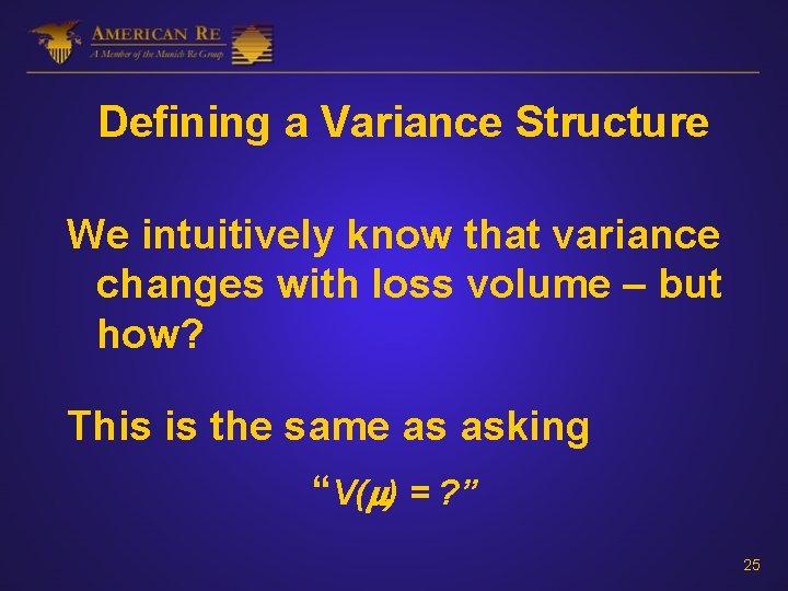
Defining a Variance Structure We intuitively know that variance changes with loss volume – but how? This is the same as asking “V( ) = ? ” 25
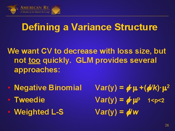
Defining a Variance Structure We want CV to decrease with loss size, but not too quickly. GLM provides several approaches: • Negative Binomial Var(y) = · +( /k)· 2 • Tweedie Var(y) = · p • Weighted L-S Var(y) = /w 1<p<2 26
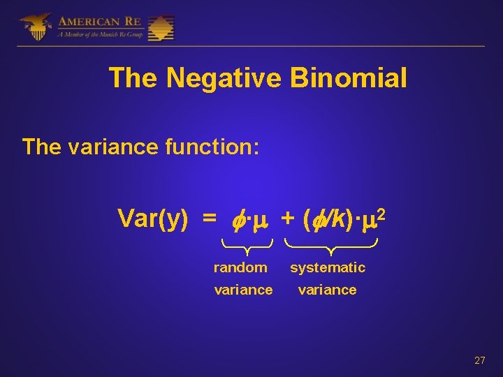
The Negative Binomial The variance function: Var(y) = · + ( /k)· 2 random systematic variance 27
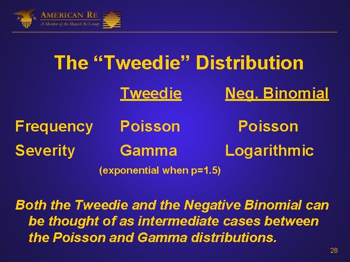
The “Tweedie” Distribution Tweedie Neg. Binomial Frequency Poisson Severity Gamma Logarithmic (exponential when p=1. 5) Both the Tweedie and the Negative Binomial can be thought of as intermediate cases between the Poisson and Gamma distributions. 28
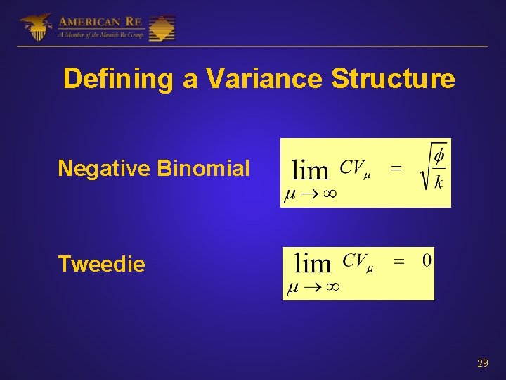
Defining a Variance Structure Negative Binomial Tweedie 29
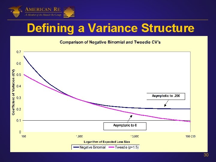
Defining a Variance Structure 30
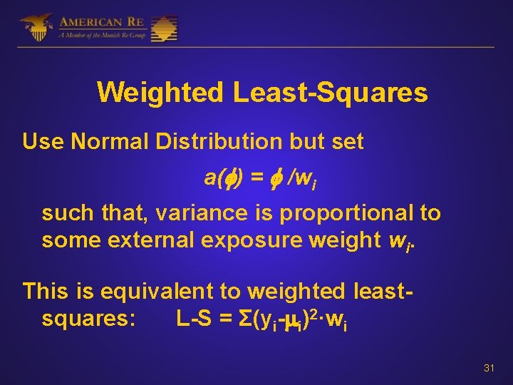
Weighted Least-Squares Use Normal Distribution but set a( ) = /wi such that, variance is proportional to some external exposure weight wi. This is equivalent to weighted leastsquares: L-S = Σ(yi- i)2·wi 31
Conclusion A model fitted to insurance data should reflect the variance structure of the phenomenon being modeled. GLM provides a flexible tool for doing this. 32
- Slides: 32