A novel functional ultrasound image based on generalized

A novel functional ultrasound image based on generalized Rayleigh scattering distribution for tissue characterization 以廣義雷利散射分佈為基礎之新世代功能性超音波影像 Po-Hsiang Tsui (崔博翔) and Chien-Cheng Chang (張建成) Division of Mechanics, Research Center for Applied Sciences, Academia Sinica 中央研究院應用科學研究中心 力學與 程科學專題中心

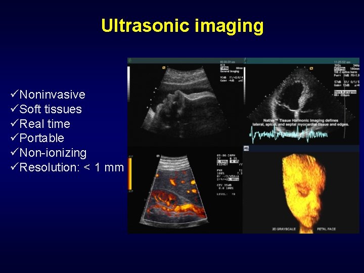
Ultrasonic imaging üNoninvasive üSoft tissues üReal time üPortable üNon-ionizing üResolution: < 1 mm

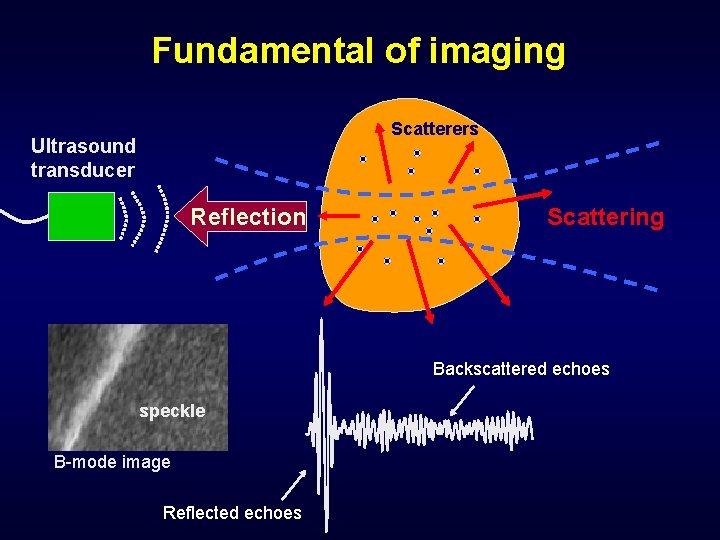
Fundamental of imaging Scatterers Ultrasound transducer Reflection Scattering Backscattered echoes speckle B-mode image Reflected echoes

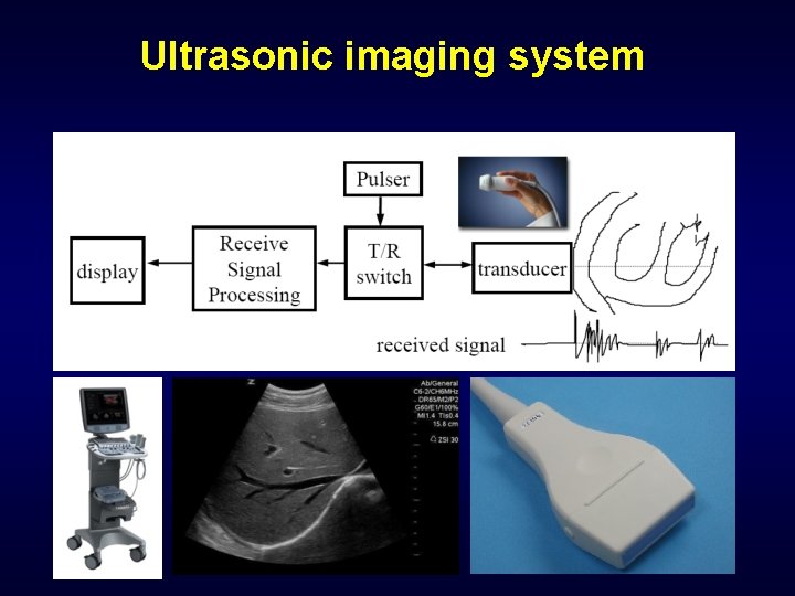
Ultrasonic imaging system

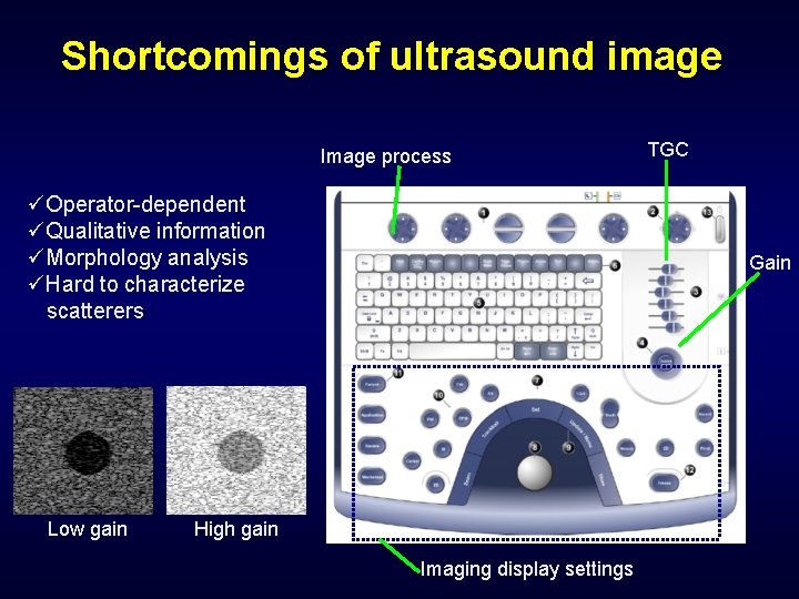
Shortcomings of ultrasound image Image process üOperator-dependent üQualitative information üMorphology analysis üHard to characterize scatterers Low gain TGC Gain High gain Imaging display settings

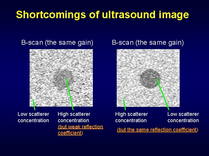
Shortcomings of ultrasound image B-scan (the same gain) Low scatterer concentration High scatterer concentration (but weak reflection coefficient) B-scan (the same gain) High scatterer concentration Low scatterer concentration (but the same reflection coefficient)

How to characterize scatterers by B-scan data?

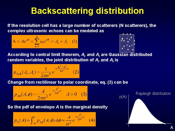
Backscattering distribution If the resolution cell has a large number of scatterers (N scatterers), the complex ultrasonic echoes can be modeled as According to central limit theorem, Ar and Ai are Gaussian distributed random variables, the joint distribution of Ar and Ai is Change from rectilinear to polar coordinate, eq. (2) can be p(A) Rayleigh distribution So the pdf of envelope A is the marginal density A

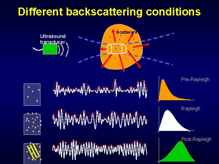
Different backscattering conditions Ultrasound transducer Scatterers Pre-Rayleigh Post-Rayleigh

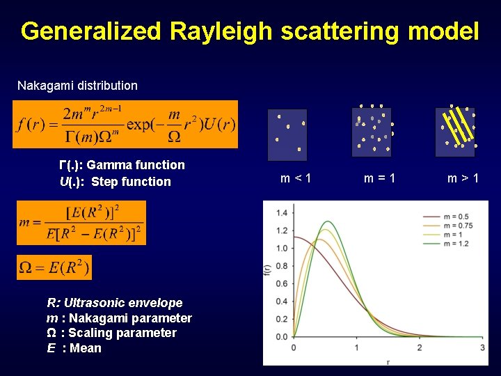
Generalized Rayleigh scattering model Nakagami distribution Γ(. ): Gamma function U(. ): Step function R: Ultrasonic envelope m : Nakagami parameter Ω : Scaling parameter E : Mean m<1 m=1 m>1

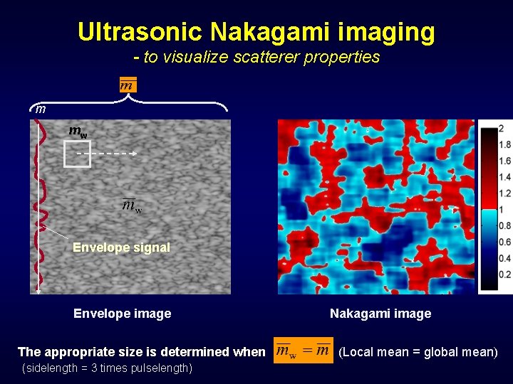
Ultrasonic Nakagami imaging - to visualize scatterer properties m mw Envelope signal Envelope image The appropriate size is determined when (sidelength = 3 times pulselength) Nakagami image (Local mean = global mean)

Simulation, animal model, and clinical experiment

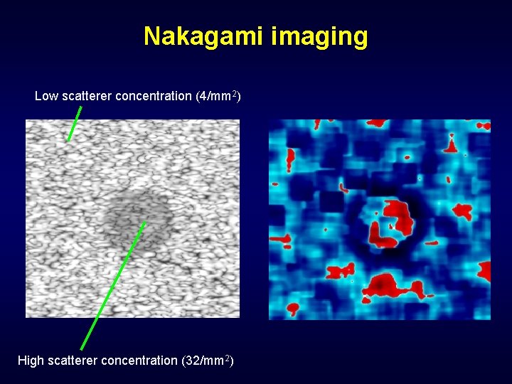
Nakagami imaging Low scatterer concentration (4/mm 2) High scatterer concentration (32/mm 2)

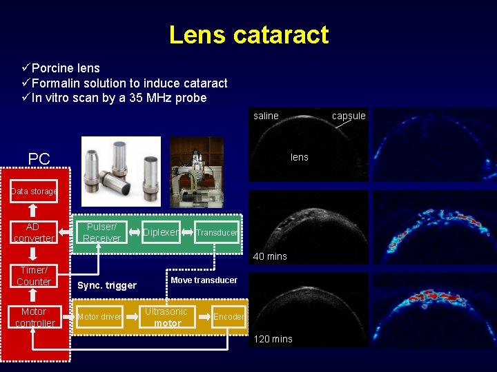
Lens cataract üPorcine lens üFormalin solution to induce cataract üIn vitro scan by a 35 MHz probe saline PC capsule lens Data storage AD converter Pulser/ Receiver Diplexer Transducer 40 mins Timer/ Counter Motor controller Sync. trigger Motor driver Move transducer Ultrasonic motor Encoder 120 mins

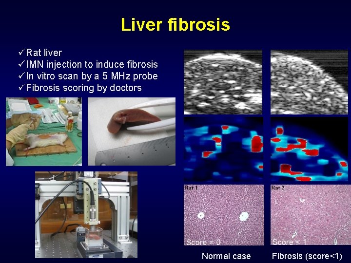
Liver fibrosis üRat liver üIMN injection to induce fibrosis üIn vitro scan by a 5 MHz probe üFibrosis scoring by doctors Normal case Fibrosis (score<1)

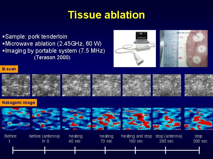
Tissue ablation §Sample: pork tenderloin §Microwave ablation (2. 45 GHz, 60 W) §Imaging by portable system (7. 5 MHz) (Terason 2000) B-scan Nakagami image Before t before (antenna) t= 0 heating 40 sec heating 70 sec heating and stop (antenna) 100 sec 280 sec stop 300 sec

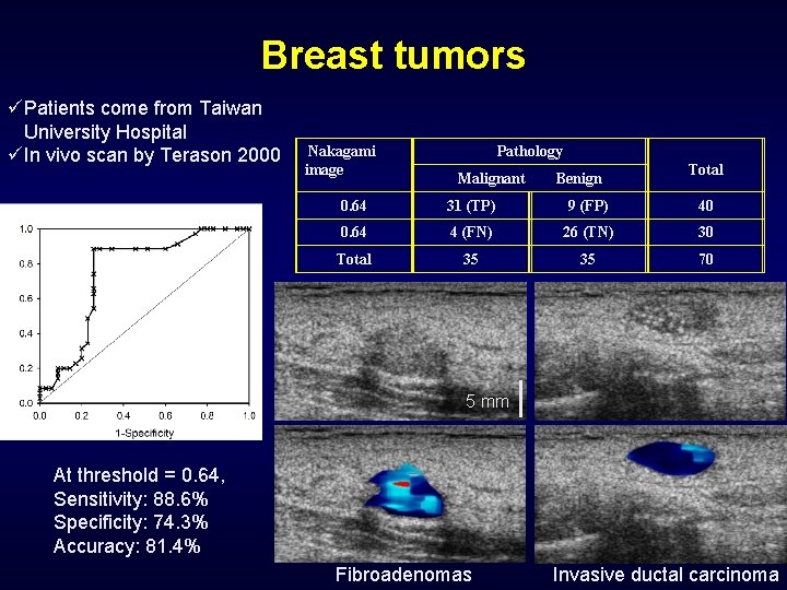
Breast tumors üPatients come from Taiwan University Hospital üIn vivo scan by Terason 2000 Nakagami image Pathology Malignant Benign Total 0. 64 31 (TP) 9 (FP) 40 0. 64 4 (FN) 26 (TN) 30 Total 35 35 70 5 mm At threshold = 0. 64, Sensitivity: 88. 6% Specificity: 74. 3% Accuracy: 81. 4% Fibroadenomas Invasive ductal carcinoma

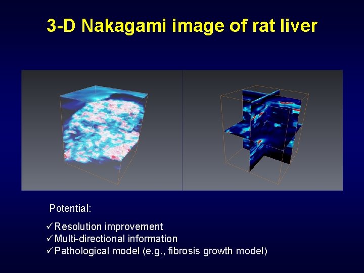
3 -D Nakagami image of rat liver Potential: üResolution improvement üMulti-directional information üPathological model (e. g. , fibrosis growth model)

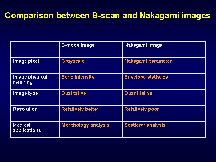
Comparison between B-scan and Nakagami images B-mode image Nakagami image Image pixel Grayscale Nakagami parameter Image physical meaning Echo intensity Envelope statistics Image type Qualitative Quantitative Resolution Relatively better Relatively poor Medical applications Morphology analysis Scatterer analysis

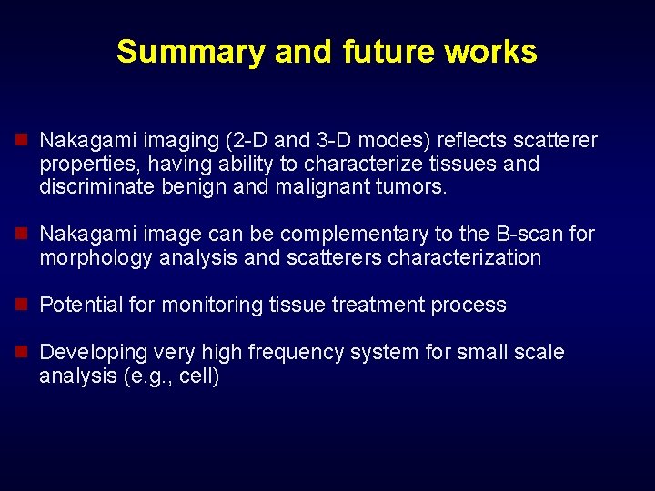
Summary and future works n Nakagami imaging (2 -D and 3 -D modes) reflects scatterer properties, having ability to characterize tissues and discriminate benign and malignant tumors. n Nakagami image can be complementary to the B-scan for morphology analysis and scatterers characterization n Potential for monitoring tissue treatment process n Developing very high frequency system for small scale analysis (e. g. , cell)

Thank you for your attention