A new model for quantifying climate episodes ATMS

“A new model for quantifying climate episodes” ATMS 790 GRADUATE SEMINAR Extreme Weather Events and Climate Ilaria Vinci 0

Content ØIntroduction • Stochastic models • Climatic episodes ØModel definition • Bivariate Distribution • BEG ØModel application • The Data ØExample • “Dust Bowl” ØConclusion ØBased on the paper: • Biondi F, Kozubowski TJ, Panorska AK. 2002. NEW MODEL FOR QUANTIFYING CLIMATE EPISODES. International Journal of Climatology 1

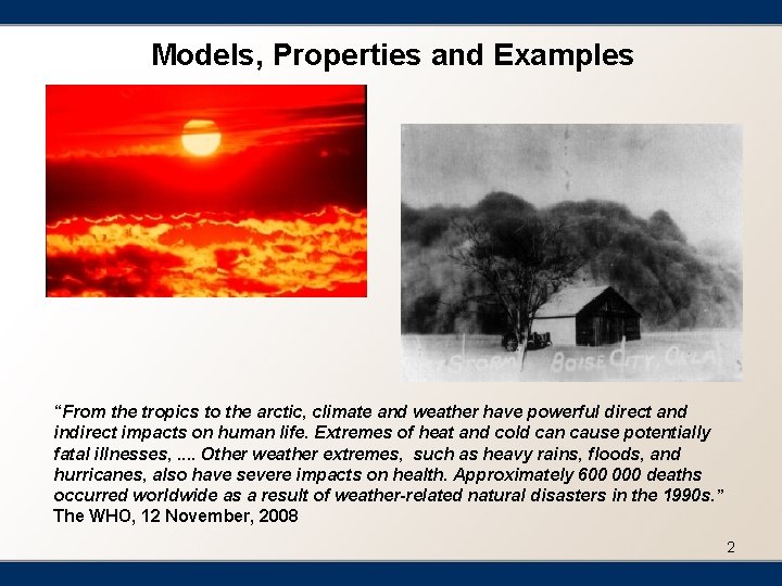
Models, Properties and Examples “From the tropics to the arctic, climate and weather have powerful direct and indirect impacts on human life. Extremes of heat and cold can cause potentially fatal illnesses, . . Other weather extremes, such as heavy rains, floods, and hurricanes, also have severe impacts on health. Approximately 600 000 deaths occurred worldwide as a result of weather-related natural disasters in the 1990 s. ” The WHO, 12 November, 2008 2

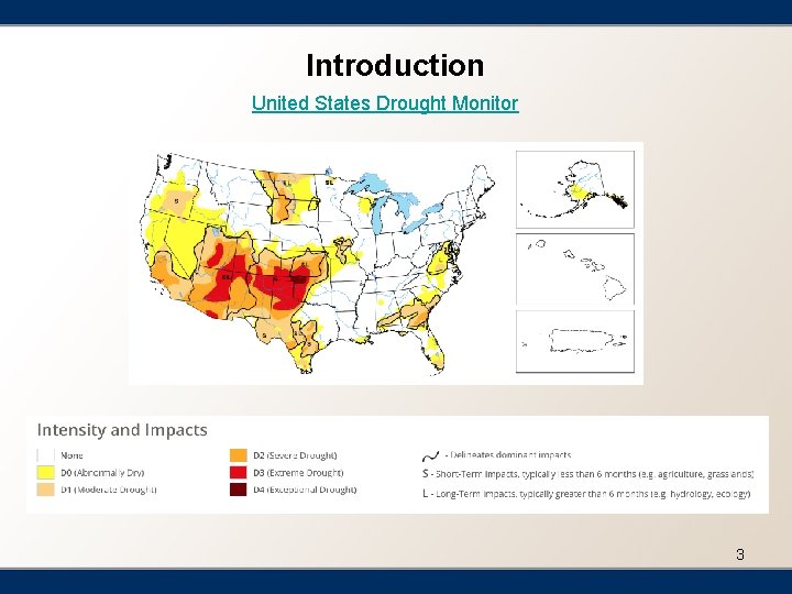
Introduction United States Drought Monitor 3

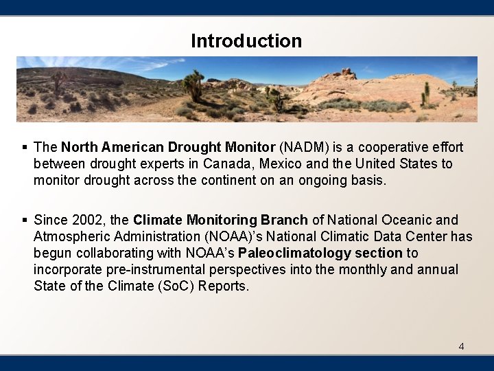
Introduction § The North American Drought Monitor (NADM) is a cooperative effort between drought experts in Canada, Mexico and the United States to monitor drought across the continent on an ongoing basis. § Since 2002, the Climate Monitoring Branch of National Oceanic and Atmospheric Administration (NOAA)’s National Climatic Data Center has begun collaborating with NOAA’s Paleoclimatology section to incorporate pre-instrumental perspectives into the monthly and annual State of the Climate (So. C) Reports. 4

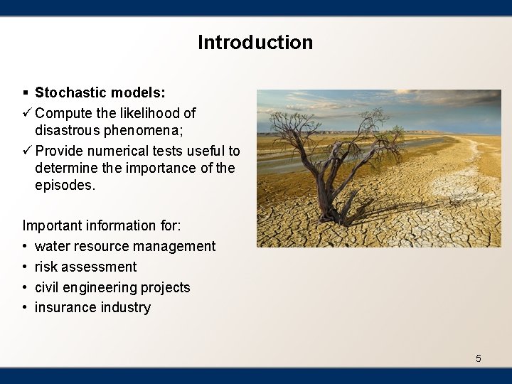
Introduction § Stochastic models: ü Compute the likelihood of disastrous phenomena; ü Provide numerical tests useful to determine the importance of the episodes. Important information for: • water resource management • risk assessment • civil engineering projects • insurance industry 5

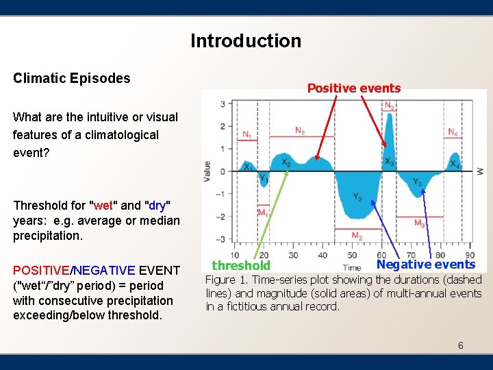
Introduction Climatic Episodes Positive events What are the intuitive or visual features of a climatological event? Threshold for "wet" and "dry" years: e. g. average or median precipitation. POSITIVE/NEGATIVE EVENT ("wet“/”dry” period) = period with consecutive precipitation exceeding/below threshold Negative events Figure 1. Time-series plot showing the durations (dashed lines) and magnitude (solid areas) of multi-annual events in a fictitious annual record. 6

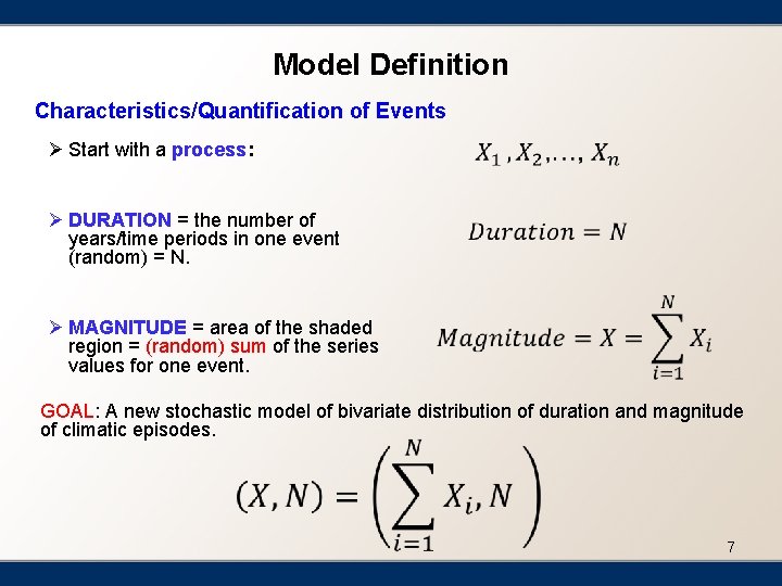
Model Definition Characteristics/Quantification of Events Ø Start with a process: Ø DURATION = the number of years/time periods in one event (random) = N. Ø MAGNITUDE = area of the shaded region = (random) sum of the series values for one event. GOAL: A new stochastic model of bivariate distribution of duration and magnitude of climatic episodes. 7

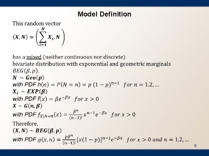
Model Definition 8

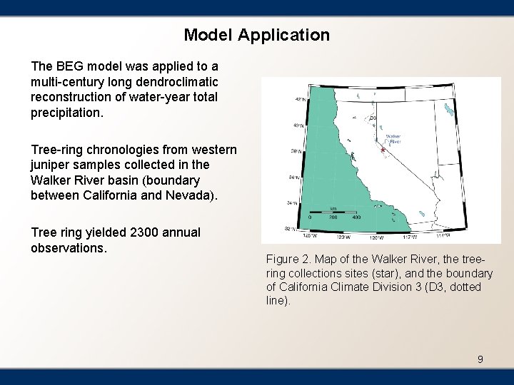
Model Application The BEG model was applied to a multi-century long dendroclimatic reconstruction of water-year total precipitation. Tree-ring chronologies from western juniper samples collected in the Walker River basin (boundary between California and Nevada). Tree ring yielded 2300 annual observations. Figure 2. Map of the Walker River, the treering collections sites (star), and the boundary of California Climate Division 3 (D 3, dotted line). 9

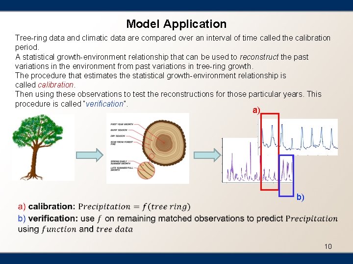
Model Application Tree-ring data and climatic data are compared over an interval of time called the calibration period. A statistical growth-environment relationship that can be used to reconstruct the past variations in the environment from past variations in tree-ring growth. The procedure that estimates the statistical growth-environment relationship is called calibration. Then using these observations to test the reconstructions for those particular years. This procedure is called “verification”. a) § b) 10

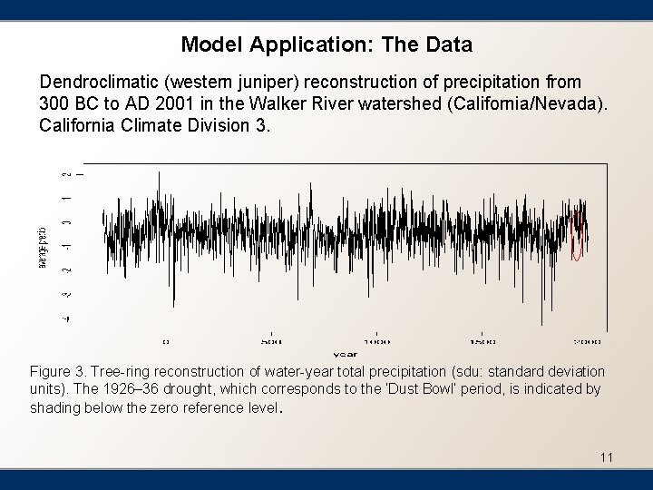
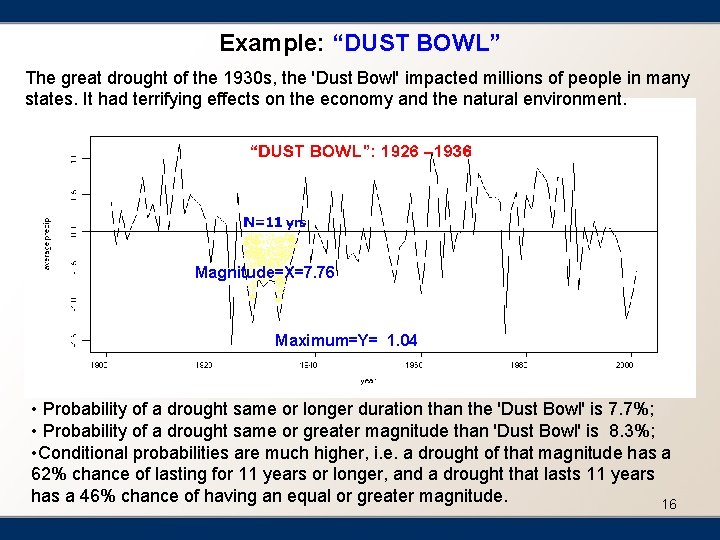
Model Application: The Data Dendroclimatic (western juniper) reconstruction of precipitation from 300 BC to AD 2001 in the Walker River watershed (California/Nevada). California Climate Division 3. Figure 3. Tree-ring reconstruction of water-year total precipitation (sdu: standard deviation units). The 1926– 36 drought, which corresponds to the ‘Dust Bowl’ period, is indicated by shading below the zero reference level. 11

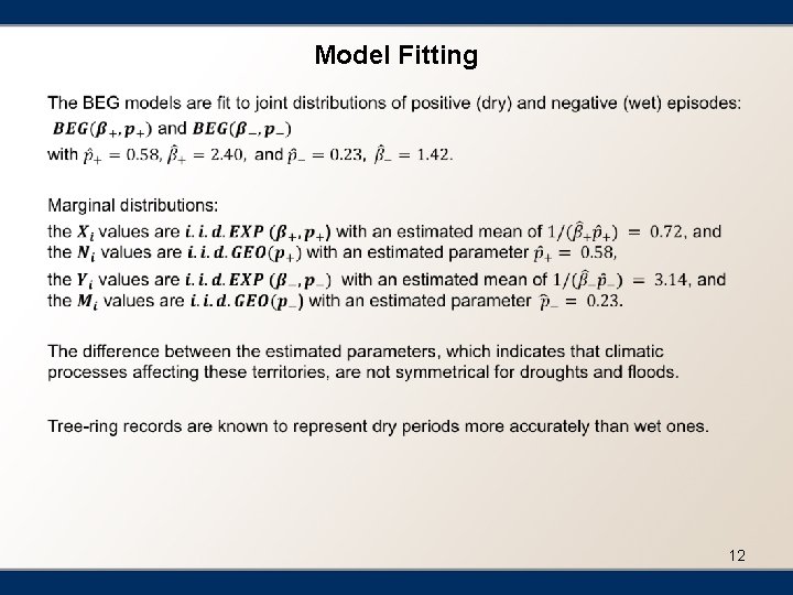
Model Fitting § 12

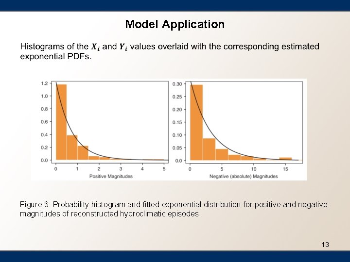
Model Application § Figure 6. Probability histogram and fitted exponential distribution for positive and negative magnitudes of reconstructed hydroclimatic episodes. 13

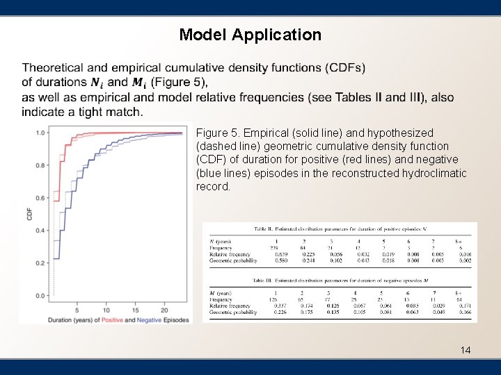
Model Application Figure 5. Empirical (solid line) and hypothesized (dashed line) geometric cumulative density function (CDF) of duration for positive (red lines) and negative (blue lines) episodes in the reconstructed hydroclimatic record. 14

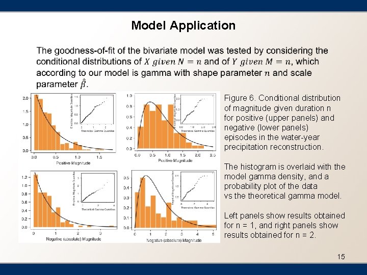
Model Application Figure 6. Conditional distribution of magnitude given duration n for positive (upper panels) and negative (lower panels) episodes in the water-year precipitation reconstruction. The histogram is overlaid with the model gamma density, and a probability plot of the data vs theoretical gamma model. Left panels show results obtained for n = 1, and right panels show results obtained for n = 2. 15

Example: “DUST BOWL” The great drought of the 1930 s, the 'Dust Bowl' impacted millions of people in many states. It had terrifying effects on the economy and the natural environment. Magnitude=X=7. 76 Maximum=Y= 1. 04 • Probability of a drought same or longer duration than the 'Dust Bowl' is 7. 7%; • Probability of a drought same or greater magnitude than 'Dust Bowl' is 8. 3%; • Conditional probabilities are much higher, i. e. a drought of that magnitude has a 62% chance of lasting for 11 years or longer, and a drought that lasts 11 years has a 46% chance of having an equal or greater magnitude. 16

Summary ØIntroduction • Stochastic models • Climatic episodes ØModel definition • Bivariate Distribution • BEG ØModel application • The Data ØExample • “Dust Bowl” 17

Conclusions v The BEG model allows to compute the likelihood of dry or wet episodes of a given duration and magnitude. We discuss that we have identified a theoretical, stochastic mechanism capable of generating the probability distributions that were empirically found to describe duration/magnitude data in several studies of climatic episodes. v The next step would be to include an additional variable that is commonly used to describe climatic episodes, i. e. the peak value, or absolute maximum, and to model the joint trivariate distribution of duration, magnitude, and peak, as well as the bivariate properties of peak and duration, and of peak and magnitude. 18

References § Biondi F, Kozubowski TJ, Panorska AK. 2002. NEW MODEL FOR QUANTIFYING CLIMATE EPISODES. International Journal of Climatology § Biondi F, Kozubowski TJ, Panorska AK. 2002. Stochastic modeling of regime shifts. Climate Research 23: 23– 30. § Kozubowski TJ, Panorska AK. In press. A mixed bivariate distribution with exponential and geometric marginals. Journal of Statistical Planning and Inference. 19

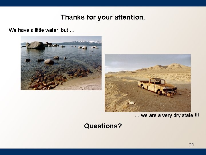
Thanks for your attention. We have a little water, but … … we are a very dry state !!! Questions? 20