A Microsegregation Model Vaughan Voller University of Minnesota



- Slides: 11

A Microsegregation Model – Vaughan Voller, University of Minnesota Process REV representative ½ arm space g solid ~ 50 mm ~0. 5 m ~5 mm Computational grid size sub-grid model column floor building 1 of 11

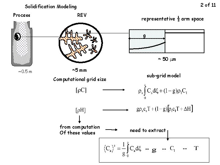
2 of 11 Solidification Modeling Process REV representative ½ arm space g solid ~ 50 mm ~0. 5 m ~5 mm Computational grid size from computation Of these values sub-grid model need to extract -- -- --

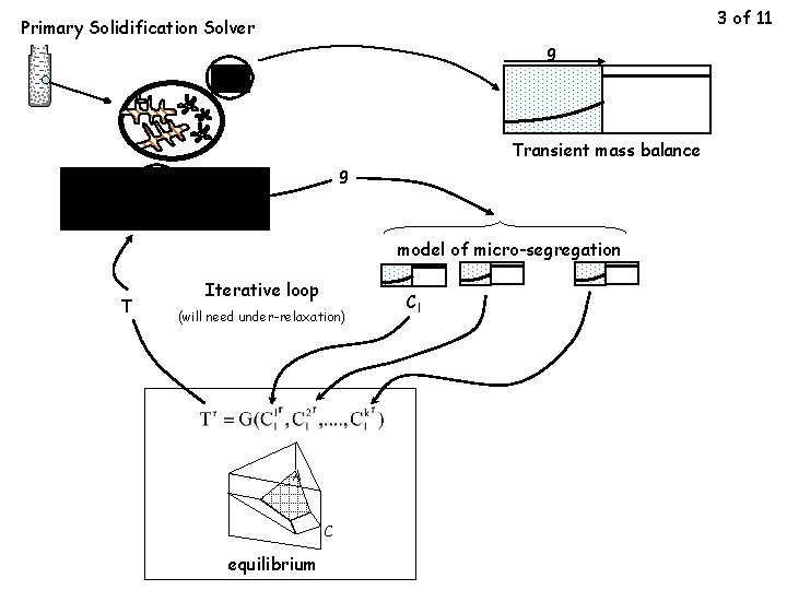
3 of 11 Primary Solidification Solver g Transient mass balance g model of micro-segregation T Iterative loop (will need under-relaxation) A C equilibrium Cl

Micro-segregation Model 4 of 11 liquid concentration due to macro-segregation alone new solid forms with lever rule on concentration transient mass balance gives liquid concentration Solute mass density before solidification Solute mass density after solidification Solute mass density of new solid (lever) q -– back-diffusion (1/s) Need an easy to use approximation For back-diffusion

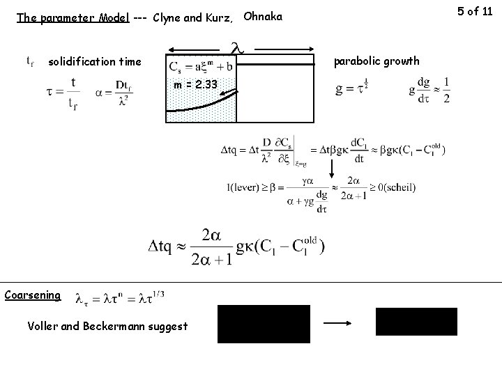
5 of 11 The parameter Model --- Clyne and Kurz, Ohnaka parabolic growth solidification time m = 2. 33 Coarsening Voller and Beckermann suggest

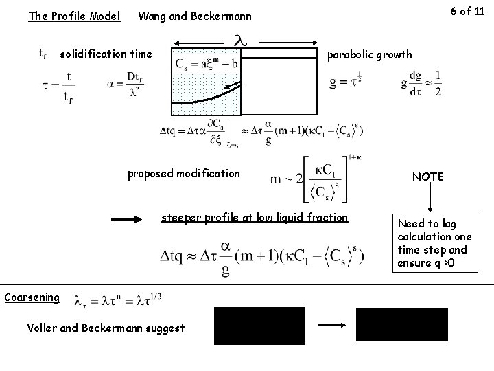
The Profile Model 6 of 11 Wang and Beckermann solidification time parabolic growth proposed modification steeper profile at low liquid fraction Coarsening Voller and Beckermann suggest NOTE Need to lag calculation one time step and ensure q >0

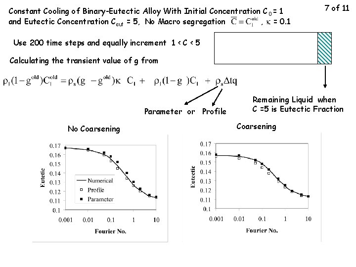
Constant Cooling of Binary-Eutectic Alloy With Initial Concentration C 0 = 1 and Eutectic Concentration Ceut = 5, No Macro segregation , k = 0. 1 7 of 11 Use 200 time steps and equally increment 1 < C < 5 Calculating the transient value of g from Parameter or Profile No Coarsening Remaining Liquid when C =5 is Eutectic Fraction Coarsening

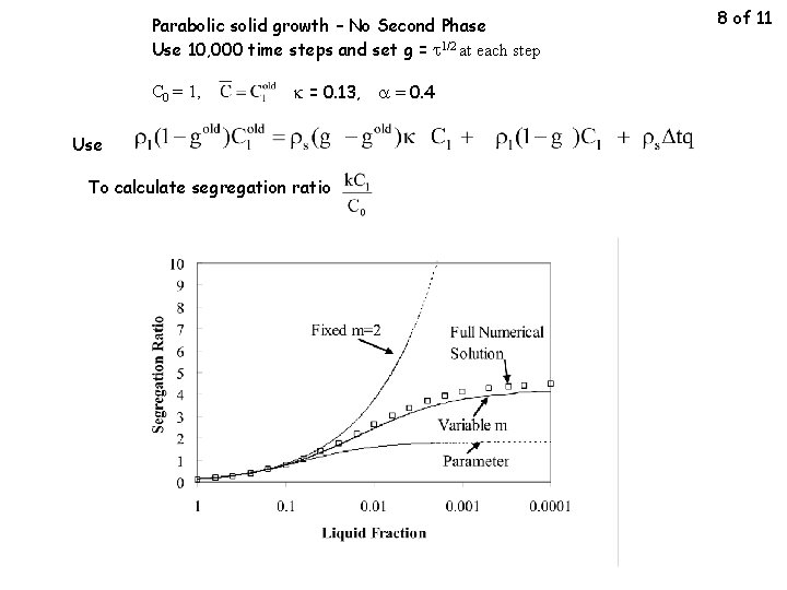
Parabolic solid growth – No Second Phase Use 10, 000 time steps and set g = t 1/2 at each step C 0 = 1, k = 0. 13, a = 0. 4 Use To calculate segregation ratio 8 of 11

Performance of Profile Model parabolic growth no second phase Prediction of segregation ratio k =0. 1 in last liquid to solidify 9 of 11 (fit exponential through last two time points) k =0. 4

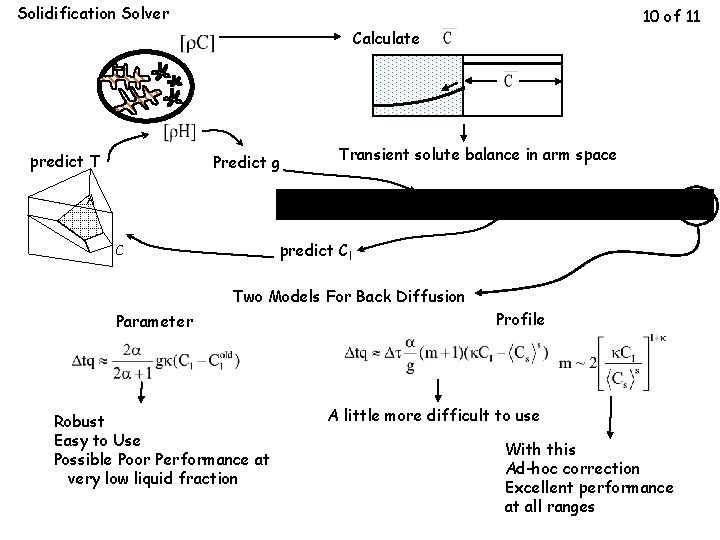
Solidification Solver 10 of 11 Calculate predict T Predict g Transient solute balance in arm space A predict Cl C Two Models For Back Diffusion Parameter Robust Easy to Use Possible Poor Performance at very low liquid fraction Profile A little more difficult to use With this Ad-hoc correction Excellent performance at all ranges

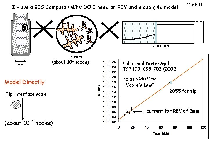
I Have a BIG Computer Why DO I need an REV and a sub grid model 11 of 11 solid ~ 50 mm . 5 m ~5 mm (about 106 nodes) Model Directly Tip-interface scale Voller and Porte-Agel, JCP 179, 698 -703 (2002 1000 20. 6667 Year “Moore’s Law” 2055 for tip current for REV of 5 mm (about 1018 nodes)