A MACHINE LEARNING APPROACH TO ANDROID MALWARE DETECTION

A MACHINE LEARNING APPROACH TO ANDROID MALWARE DETECTION 1 JUSTIN SAHS AND PROF. LATIFUR KHAN

The Problem 2 Smartphones represent a significant and growing proportion of computing devices Android in particular is the fastest growing smartphone platform, and has 52. 5% market share* The power of the Android platform allows for applications providing a variety of services, including sensitive services like banking This power can also be leveraged by malware *http: //www. gartner. com/it/page. jsp? id=1848514

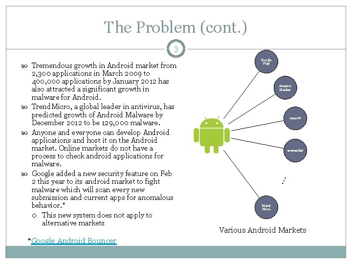
The Problem (cont. ) 3 2, 300 applications in March 2009 to 400, 000 applications by January 2012 has also attracted a significant growth in malware for Android. Trend. Micro, a global leader in antivirus, has predicted growth of Android Malware by December 2012 to be 129, 000 malware. Anyone and everyone can develop Android applications and host it on the Android market. Online markets do not have a process to check android applications for malware. Google added a new security feature on Feb 2 this year to its android market to fight malware which will scan every new submission and current apps for anomalous behavior. * This new system does not apply to alternative markets *Google Android Bouncer Google Play Amazon Market mmovv eoemarket … Tremendous growth in Android market from Many More Various Android Markets

The Problem (cont. ) 4 Smartphones are becoming increasingly ubiquitous. A report from Gartner shows that there were over 100 million smart phones sold in the first quarter of 2011, an increase of 85% over the first quarter of 2010*. Malware often disguise themselves as normal applications Malware can cause financial loss, theft of private information Users need robust malware detection software *http: //www. gartner. com/it/page. jsp? id=1689814

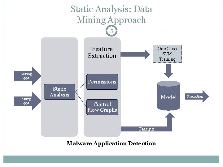
Static Analysis: Data Mining Approach 5 Feature Extraction Training Apps Testing Apps One Class SVM Training Permissions Static Analysis Model Control Flow Graphs Testing Malware Application Detection Prediction

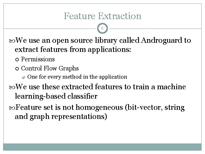
Feature Extraction 6 We use an open source library called Androguard to extract features from applications: Permissions Control Flow Graphs One for every method in the application We use these extracted features to train a machine learning-based classifier Feature set is not homogeneous (bit-vector, string and graph representations)

Feature Extraction: Acquiring Applications 7 APK files are Android package files. Applications that are packaged as APKs can be installed in any compatible android device. Benign APK files were harvested from the official Android Market using the android-market-api, * in addition to a collection of known malware We used 2, 172 APK files in our analysis. *http: //code. google. com/p/android-market-api/

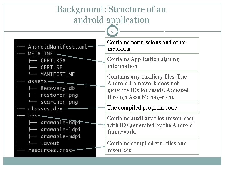
Background: Structure of an android application 8 Contains permissions and other metadata Contains Application signing information Contains any auxiliary files. The Android framework does not generate IDs for assets. Accessed through Asset. Manager api. The compiled program code Contains auxiliary files (resources) with IDs generated by the Android framework. Contains compiled xml files and resources.

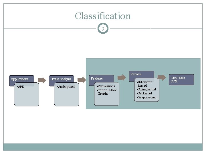
Classification 9 Kernels Applications • APK Static Analysis • Androguard Features • Permissions • Control Flow Graphs • Bit-vector kernel • String kernel • Set kernel • Graph kernel One-Class SVM

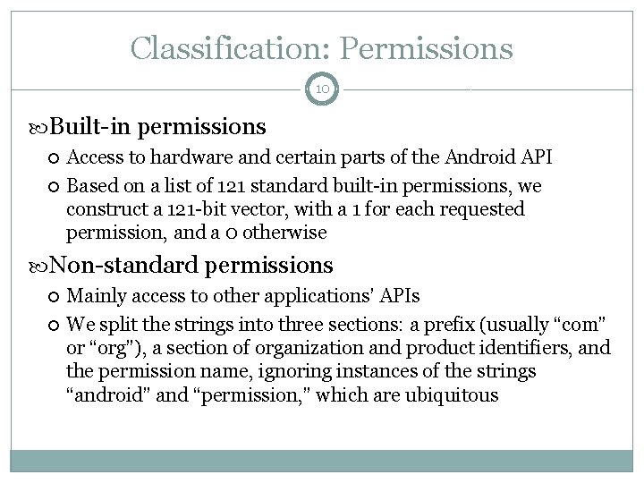
Classification: Permissions 10 Built-in permissions Access to hardware and certain parts of the Android API Based on a list of 121 standard built-in permissions, we construct a 121 -bit vector, with a 1 for each requested permission, and a 0 otherwise Non-standard permissions Mainly access to other applications’ APIs We split the strings into three sections: a prefix (usually “com” or “org”), a section of organization and product identifiers, and the permission name, ignoring instances of the strings “android” and “permission, ” which are ubiquitous

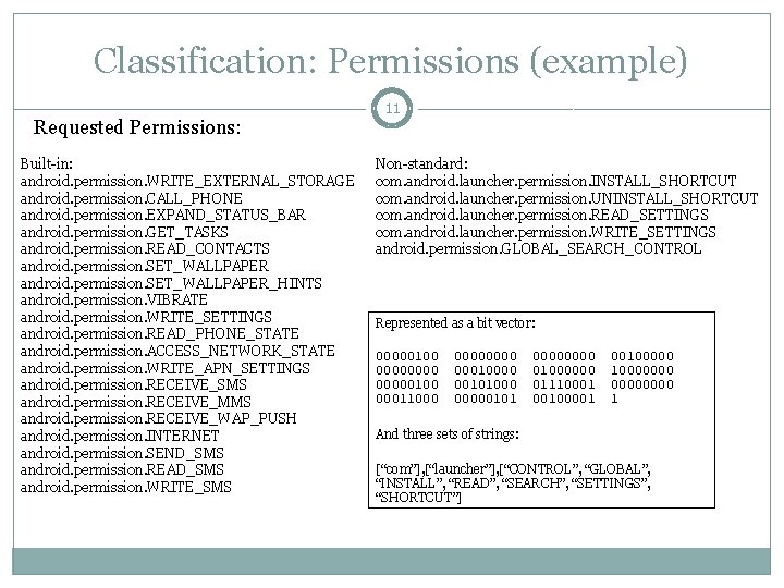
Classification: Permissions (example) Requested Permissions: Built-in: android. permission. WRITE_EXTERNAL_STORAGE android. permission. CALL_PHONE android. permission. EXPAND_STATUS_BAR android. permission. GET_TASKS android. permission. READ_CONTACTS android. permission. SET_WALLPAPER_HINTS android. permission. VIBRATE android. permission. WRITE_SETTINGS android. permission. READ_PHONE_STATE android. permission. ACCESS_NETWORK_STATE android. permission. WRITE_APN_SETTINGS android. permission. RECEIVE_SMS android. permission. RECEIVE_MMS android. permission. RECEIVE_WAP_PUSH android. permission. INTERNET android. permission. SEND_SMS android. permission. READ_SMS android. permission. WRITE_SMS 11 Non-standard: com. android. launcher. permission. INSTALL_SHORTCUT com. android. launcher. permission. UNINSTALL_SHORTCUT com. android. launcher. permission. READ_SETTINGS com. android. launcher. permission. WRITE_SETTINGS android. permission. GLOBAL_SEARCH_CONTROL Represented as a bit vector: 00000100 00000100 00011000 0000 00010000 00101000 00000101 0000 01000000 01110001 0010000000 0000 1 And three sets of strings: [“com”], [“launcher”], [“CONTROL”, “GLOBAL”, “INSTALL”, “READ”, “SEARCH”, “SETTINGS”, “SHORTCUT”]

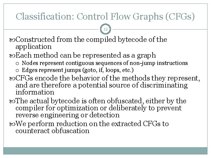
Classification: Control Flow Graphs (CFGs) 12 Constructed from the compiled bytecode of the application Each method can be represented as a graph Nodes represent contiguous sequences of non-jump instructions Edges represent jumps (goto, if, loops, etc. ) CFGs encode the behavior of the methods they represent, and are therefore a potential source of discriminating information The actual bytecode is often obfuscated, either by the compiler for optimization or deliberately to prevent reverse engineering or detection We perform reduction on the extracted CFGs to counteract obfuscation

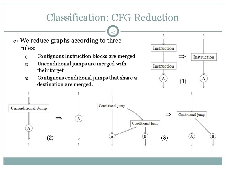
Classification: CFG Reduction 13 We reduce graphs according to three rules: 1) 2) 3) Contiguous instruction blocks are merged Unconditional jumps are merged with their target Contiguous conditional jumps that share a destination are merged. (2) (1) (3)

Classification: Training and Testing 14 Once we have extracted our feature representations, we use them to train a One-Class Support Vector Machine (1 C-SVM) The 1 C-SVM is designed to detect test examples that are significantly different than the training data We have far more examples of benign applications than malware to train on

One Class SVM (1 C-SVM) 15 A Support Vector Machine (SVM) finds the maximum- margin separating hyperplane between the positive and negative training examples in some feature space i. e. it maximizes the distance between the hyperplane and the closest examples from each class The SVM uses comparison functions called kernels to map each extracted feature into a high-dimensional feature space The linear separation of the data in the feature space may correspond to a very non-linear separation of the original data Each kernel takes two feature representations as input and outputs a number that measures similarity

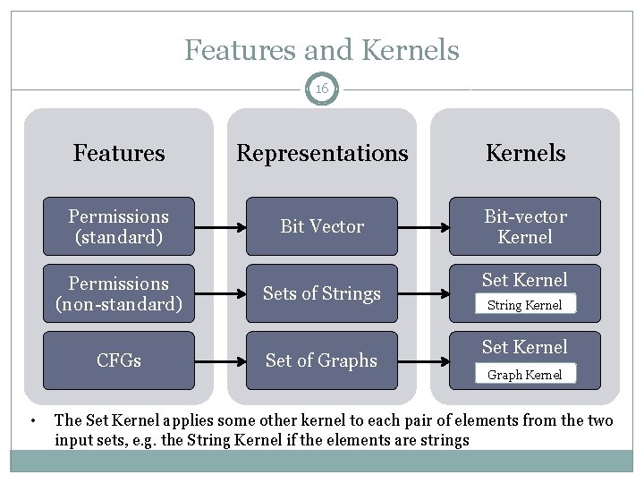
Features and Kernels 16 Features Representations Kernels Permissions (standard) Bit Vector Bit-vector Kernel Permissions (non-standard) CFGs • Sets of Strings Set of Graphs Set Kernel String Kernel Set Kernel Graph Kernel The Set Kernel applies some other kernel to each pair of elements from the two input sets, e. g. the String Kernel if the elements are strings

Classification: Training and Testing (cont. ) 17 We use a data mining library, scikit-learn (http: //scikit-learn. org/), which implements a convenient wrapper around the popular LIBSVM (http: //www. csie. ntu. edu. tw/~cjlin/libsvm/) The use of a SVM requires specialized functions called kernels that are used to compare features between applications We implement these kernels ourselves

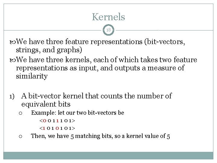
Kernels 18 We have three feature representations (bit-vectors, strings, and graphs) We have three kernels, each of which takes two feature representations as input, and outputs a measure of similarity 1) A bit-vector kernel that counts the number of equivalent bits Example: let our two bit-vectors be <0 0 1 1 1 0 1> <1 0 1 0 1> Then, we have 5 matching bits, so a kernel value of 5

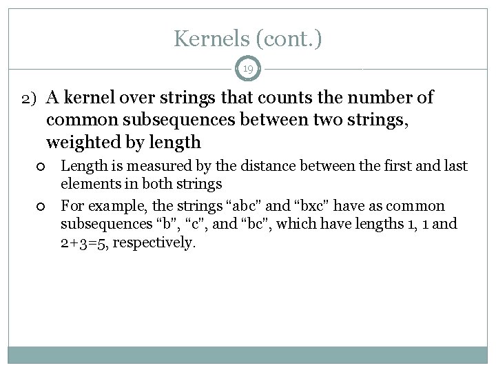
Kernels (cont. ) 19 2) A kernel over strings that counts the number of common subsequences between two strings, weighted by length Length is measured by the distance between the first and last elements in both strings For example, the strings “abc” and “bxc” have as common subsequences “b”, “c”, and “bc”, which have lengths 1, 1 and 2+3=5, respectively.

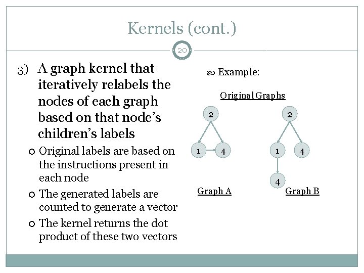
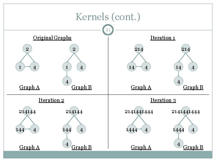
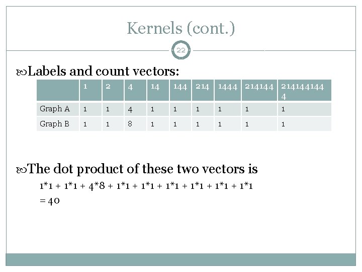
Kernels (cont. ) 20 3) A graph kernel that Example: iteratively relabels the nodes of each graph based on that node’s children’s labels Original labels are based on the instructions present in each node The generated labels are counted to generate a vector The kernel returns the dot product of these two vectors Original Graphs 2 1 2 4 Graph A 1 4 4 Graph B

Kernels (cont. ) 21 Original Graphs 2 1 Iteration 1 2 4 1 4 Graph A 214 4 Graph B 14 214 4 144 4 Graph A Iteration 2 214144 14 4 Graph B Iteration 3 214144 4 4 Graph B 2141441444 4 Graph A 4 4 Graph B

Kernels (cont. ) 22 Labels and count vectors: 1 2 4 14 144 214 1444 214144144 4 Graph A 1 1 4 1 1 1 Graph B 1 1 8 1 1 1 The dot product of these two vectors is 1*1 + 4*8 + 1*1 + 1*1 = 40

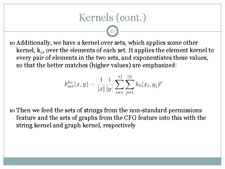
Kernels (cont. ) 23 Additionally, we have a kernel over sets, which applies some other kernel, k 0, over the elements of each set. It applies the element kernel to every pair of elements in the two sets, and exponentiates these values, so that the better matches (higher values) are emphasized: Then we feed the sets of strings from the non-standard permissions feature and the sets of graphs from the CFG feature into this with the string kernel and graph kernel, respectively

Kernels (cont. ) 24 Each of these kernel values are normalized, then summed to form the final kernel value One such value is calculated for every pair of training examples, generating a kernel matrix The kernel matrix is used to train the 1 C-SVM During testing, one value is calculated for each pair of training and testing examples.

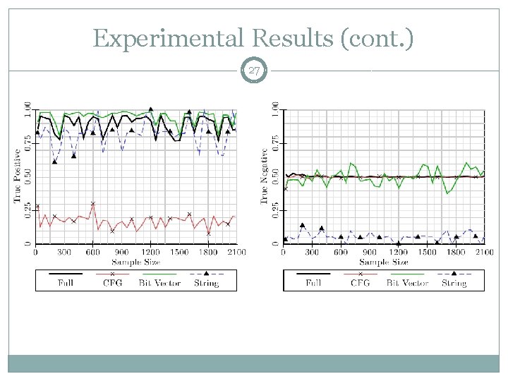
Experimental Results 25 We tested our system with 2081 benign applications and 91 malicious applications The system correctly classifies approximately 90% of malware, but only correctly classifies approximately 50% of benign applications We also tested against each of the individual features alone

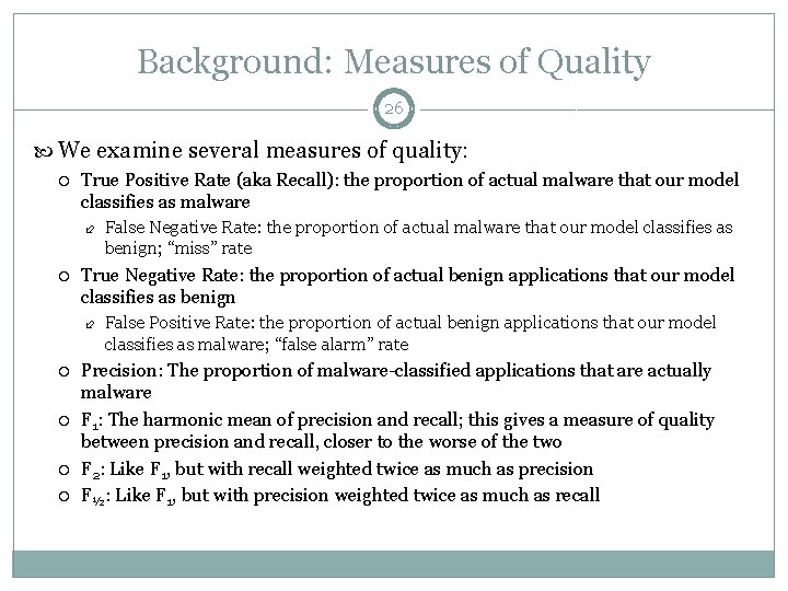
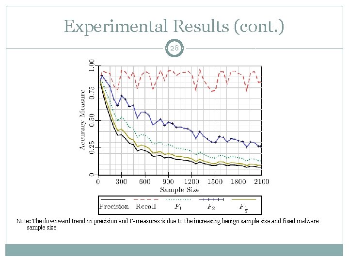
Background: Measures of Quality 26 We examine several measures of quality: True Positive Rate (aka Recall): the proportion of actual malware that our model classifies as malware True Negative Rate: the proportion of actual benign applications that our model classifies as benign False Negative Rate: the proportion of actual malware that our model classifies as benign; “miss” rate False Positive Rate: the proportion of actual benign applications that our model classifies as malware; “false alarm” rate Precision: The proportion of malware-classified applications that are actually malware F 1: The harmonic mean of precision and recall; this gives a measure of quality between precision and recall, closer to the worse of the two F 2: Like F 1, but with recall weighted twice as much as precision F½: Like F 1, but with precision weighted twice as much as recall

Experimental Results (cont. ) 27

Experimental Results (cont. ) 28 Note: The downward trend in precision and F-measures is due to the increasing benign sample size and fixed malware sample size

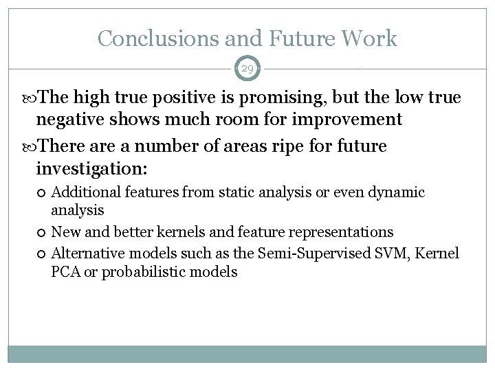
Conclusions and Future Work 29 The high true positive is promising, but the low true negative shows much room for improvement There a number of areas ripe for future investigation: Additional features from static analysis or even dynamic analysis New and better kernels and feature representations Alternative models such as the Semi-Supervised SVM, Kernel PCA or probabilistic models