A LEVEL PHYSICS Year 1 Calculating g practical

A LEVEL PHYSICS Year 1 Calculating ‘g’ practical A* A B C • Determination of g by free fall method. • Able to identify random and systematic errors in the experiment and suggest ways to remove them. • Determine g from a graph. B/C Target A/A* Target EP EP EP

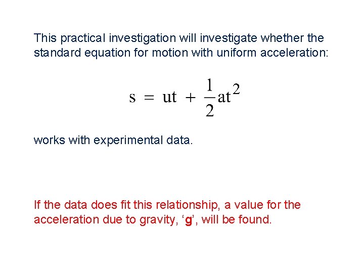
This practical investigation will investigate whether the standard equation for motion with uniform acceleration: works with experimental data. If the data does fit this relationship, a value for the acceleration due to gravity, ‘g’, will be found.

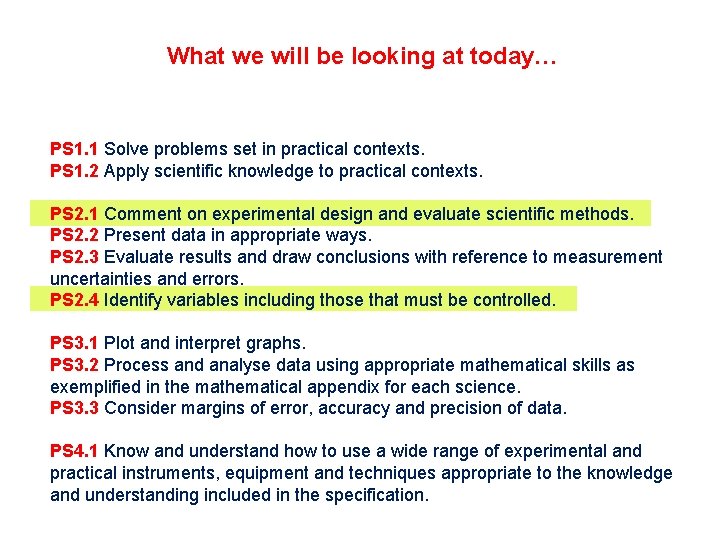
What we will be looking at today… PS 1. 1 Solve problems set in practical contexts. PS 1. 2 Apply scientific knowledge to practical contexts. PS 2. 1 Comment on experimental design and evaluate scientific methods. PS 2. 2 Present data in appropriate ways. PS 2. 3 Evaluate results and draw conclusions with reference to measurement uncertainties and errors. PS 2. 4 Identify variables including those that must be controlled. PS 3. 1 Plot and interpret graphs. PS 3. 2 Process and analyse data using appropriate mathematical skills as exemplified in the mathematical appendix for each science. PS 3. 3 Consider margins of error, accuracy and precision of data. PS 4. 1 Know and understand how to use a wide range of experimental and practical instruments, equipment and techniques appropriate to the knowledge and understanding included in the specification.

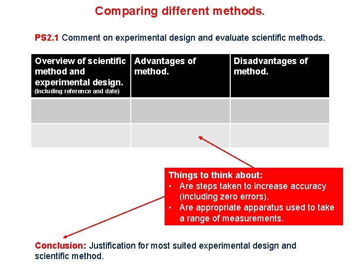
Comparing different methods. PS 2. 1 Comment on experimental design and evaluate scientific methods. Overview of scientific Advantages of method and method. experimental design. Disadvantages of method. (Including reference and date) Things to think about: • Are steps taken to increase accuracy (including zero errors). • Are appropriate apparatus used to take a range of measurements. Conclusion: Justification for most suited experimental design and scientific method.

What we will be looking at today… PS 1. 1 Solve problems set in practical contexts. PS 1. 2 Apply scientific knowledge to practical contexts. PS 2. 1 Comment on experimental design and evaluate scientific methods. PS 2. 2 Present data in appropriate ways. PS 2. 3 Evaluate results and draw conclusions with reference to measurement uncertainties and errors. PS 2. 4 Identify variables including those that must be controlled. PS 3. 1 Plot and interpret graphs. PS 3. 2 Process and analyse data using appropriate mathematical skills as exemplified in the mathematical appendix for each science. PS 3. 3 Consider margins of error, accuracy and precision of data. PS 4. 1 Know and understand how to use a wide range of experimental and practical instruments, equipment and techniques appropriate to the knowledge and understanding included in the specification.

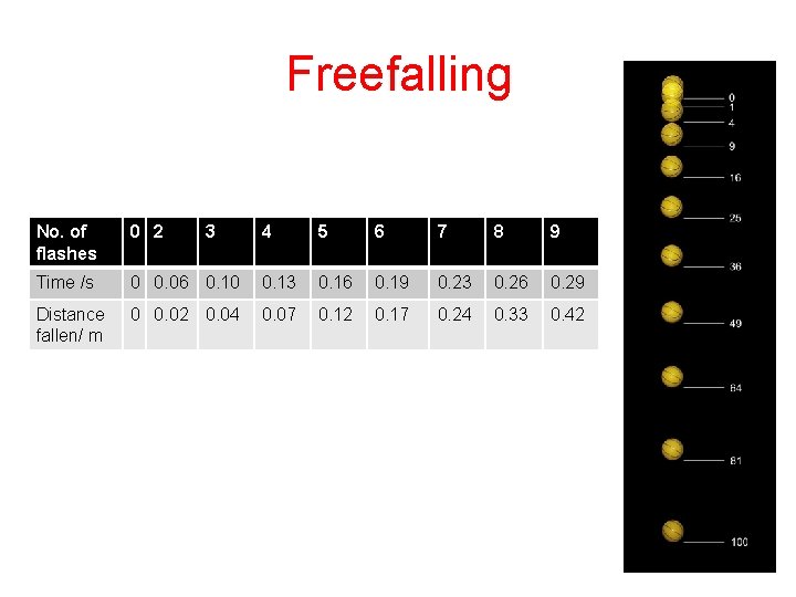
Freefalling No. of flashes 0 2 Time /s Distance fallen/ m 3 4 5 6 7 8 9 0 0. 06 0. 10 0. 13 0. 16 0. 19 0. 23 0. 26 0. 29 0 0. 02 0. 04 0. 07 0. 12 0. 17 0. 24 0. 33 0. 42

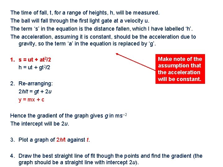
The time of fall, t, for a range of heights, h, will be measured. The ball will fall through the first light gate at a velocity u. The term ‘s’ in the equation is the distance fallen, which I have labelled ‘h’. The acceleration, assuming it is constant, should be the acceleration due to gravity, so the term ‘a’ in the equation is replaced by ‘g’. 1. s = ut + at 2/2 h = ut + gt 2/2 2. Re-arranging: 2 h/t = gt + 2 u y = mx + c Make note of the assumption that the acceleration will be constant. Hence the gradient of the graph gives g in ms– 2 The intercept will be 2 u. 3. Plot a graph of 2 h/t against t. 4. Draw the best straight line of fit though the points and find the gradient (the graph should be a straight line with intercept 2 u).

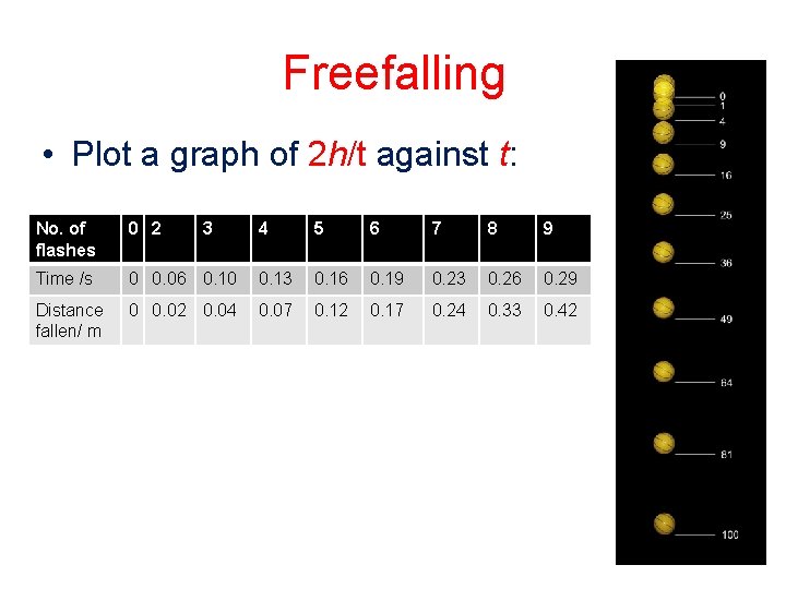
Freefalling • Plot a graph of 2 h/t against t: No. of flashes 0 2 Time /s Distance fallen/ m 3 4 5 6 7 8 9 0 0. 06 0. 10 0. 13 0. 16 0. 19 0. 23 0. 26 0. 29 0 0. 02 0. 04 0. 07 0. 12 0. 17 0. 24 0. 33 0. 42

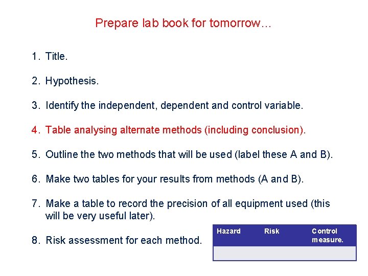
Prepare lab book for tomorrow… 1. Title. 2. Hypothesis. 3. Identify the independent, dependent and control variable. 4. Table analysing alternate methods (including conclusion). 5. Outline the two methods that will be used (label these A and B). 6. Make two tables for your results from methods (A and B). 7. Make a table to record the precision of all equipment used (this will be very useful later). 8. Risk assessment for each method. Hazard Risk Control measure.

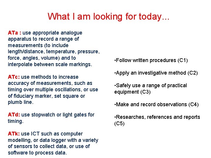
What I am looking for today. . . ATa : use appropriate analogue apparatus to record a range of measurements (to include length/distance, temperature, pressure, force, angles, volume) and to interpolate between scale markings. ATc: use methods to increase accuracy of measurements, such as timing over multiple oscillations, or use of fiduciary marker, set square or plumb line. ATd: use stopwatch or light gates for timing. ATk: use ICT such as computer modelling, or data logger with a variety of sensors to collect data, or use of software to process data. • Follow written procedures (C 1) • Apply an investigative method (C 2) • Safely use a range of practical equipment (C 3) • Make and record observations (C 4) • Researches, references and reports (C 5)

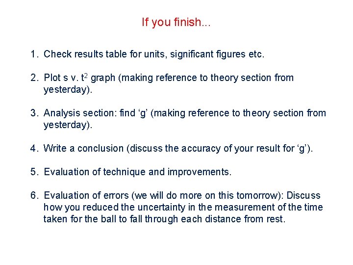
If you finish. . . 1. Check results table for units, significant figures etc. 2. Plot s v. t 2 graph (making reference to theory section from yesterday). 3. Analysis section: find ‘g’ (making reference to theory section from yesterday). 4. Write a conclusion (discuss the accuracy of your result for ‘g’). 5. Evaluation of technique and improvements. 6. Evaluation of errors (we will do more on this tomorrow): Discuss how you reduced the uncertainty in the measurement of the time taken for the ball to fall through each distance from rest.

Evaluation of errors Where do our errors comes from?

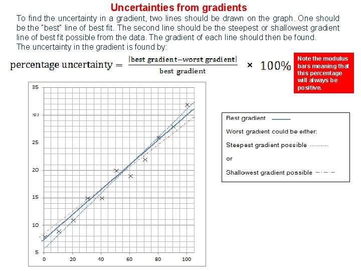
Uncertainties from gradients To find the uncertainty in a gradient, two lines should be drawn on the graph. One should be the “best” line of best fit. The second line should be the steepest or shallowest gradient line of best fit possible from the data. The gradient of each line should then be found. The uncertainty in the gradient is found by: × Note the modulus bars meaning that this percentage will always be positive.

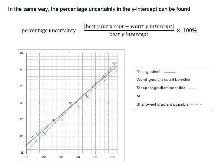
In the same way, the percentage uncertainty in the y-intercept can be found:

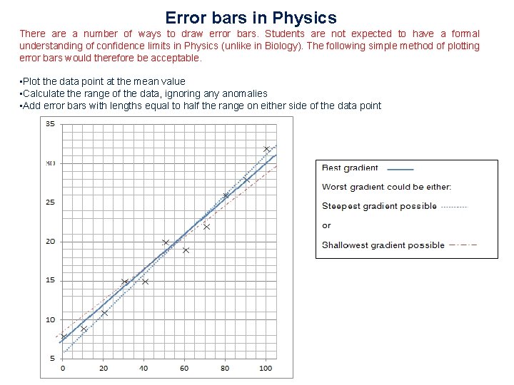
Error bars in Physics There a number of ways to draw error bars. Students are not expected to have a formal understanding of confidence limits in Physics (unlike in Biology). The following simple method of plotting error bars would therefore be acceptable. • Plot the data point at the mean value • Calculate the range of the data, ignoring any anomalies • Add error bars with lengths equal to half the range on either side of the data point

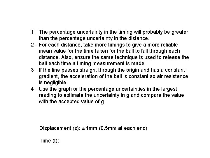
1. Compare the percentage uncertainty in the smallest distance and time measurements. 2. Discuss how you reduced the uncertainty in the measurement of the time taken for the ball to fall through each distance from rest. 3. What conclusions can you draw from your results? 4. Discuss the accuracy of your result for g.

1. The percentage uncertainty in the timing will probably be greater than the percentage uncertainty in the distance. 2. For each distance, take more timings to give a more reliable mean value for the time taken for the ball to fall through each distance. Also, ensure the same technique is used to release the ball each time a timing measurement is made. 3. If the line passes straight through the origin and has a constant gradient, the acceleration of the ball is constant so air resistance is negligible. 4. Use the graph or the percentage uncertainties in the largest reading to estimate the uncertainty in g and compare the value with the accepted value of g. Displacement (s): ± 1 mm (0. 5 mm at each end) Time (t):

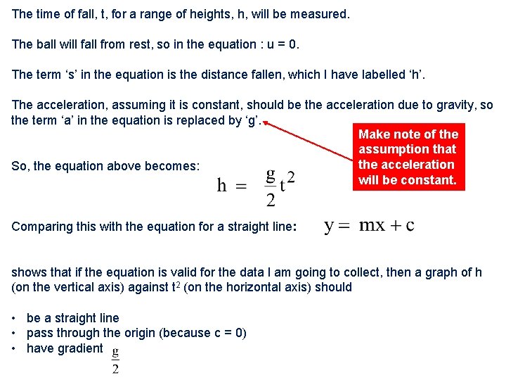
The time of fall, t, for a range of heights, h, will be measured. The ball will fall from rest, so in the equation : u = 0. The term ‘s’ in the equation is the distance fallen, which I have labelled ‘h’. The acceleration, assuming it is constant, should be the acceleration due to gravity, so the term ‘a’ in the equation is replaced by ‘g’. Make note of the assumption that the acceleration So, the equation above becomes: will be constant. Comparing this with the equation for a straight line: shows that if the equation is valid for the data I am going to collect, then a graph of h (on the vertical axis) against t 2 (on the horizontal axis) should • be a straight line • pass through the origin (because c = 0) • have gradient