A Lecture Presentation in Power Point to accompany

A Lecture Presentation in Power. Point to accompany Exploring Economics Second Edition by Robert L. Sexton Copyright © 2002 Thomson Learning, Inc. Thomson Learning™ is a trademark used herein under license. ALL RIGHTS RESERVED. Instructors of classes adopting EXPLORING ECONOMICS, Second Edition by Robert L. Sexton as an assigned textbook may reproduce material from this publication for classroom use or in a secure electronic network environment that prevents downloading or reproducing the copyrighted material. Otherwise, no part of this work covered by the copyright hereon may be reproduced or used in any form or by any means—graphic, electronic, or mechanical, including, but not limited to, photocopying, recording, taping, Web distribution, information networks, or information storage and retrieval systems—without the written permission of the publisher. Printed in the United States of America ISBN 0030342333 Copyright © 2002 by Thomson Learning, Inc.

Chapter 9 Perfect Competition Copyright © 2002 by Thomson Learning, Inc.

9. 1 A Perfectly Competitive Market n Economists have identified four different market structures in which firms operate: n n n perfect competition, monopoly, monopolistic competition, and oligopoly. Each structure has key characteristics, but it is sometimes difficult to decide which structure a given firm or industry most appropriately fits. Copyright © 2002 by Thomson Learning, Inc.

9. 1 A Perfectly Competitive Market n At one end of the continuum of market environments is pure monopoly. n n There is a single seller. The seller sets the price that will maximize its profits. Copyright © 2002 by Thomson Learning, Inc.

9. 1 A Perfectly Competitive Market n Monopolistic competition falls between perfect competition and monopoly; firms have elements of both competition and monopoly power. n n Each firm's product is differentiated from competitors’, so each has some monopoly power. However, because there are so many competitors, it also has an element of competitive markets. Copyright © 2002 by Thomson Learning, Inc.

9. 1 A Perfectly Competitive Market n Oligopoly also falls between perfect competition and monopoly, where a few firms produce similar or identical goods, as opposed to one firm or many. n n Unlike monopoly, oligopoly allows for some competition between firms. Unlike competition, individual firms have a significant share of the total market for the good being produced. Copyright © 2002 by Thomson Learning, Inc.

9. 1 A Perfectly Competitive Market n n An oligopolist is very conscious of the actions of competing firms, and its behavior is closely related to that of its competitors. An oligopolist does have some control over price and thus is a price searcher. Copyright © 2002 by Thomson Learning, Inc.

9. 1 A Perfectly Competitive Market n At the other end of the spectrum, perfect competition involves n n n a large number of buyers and sellers, a homogeneous (standardized) product, and easy market entry and exit. Copyright © 2002 by Thomson Learning, Inc.

9. 1 A Perfectly Competitive Market n n In perfect competition, no single firm produces more than an extremely small proportion of output, so no firm can influence the market price or quantity. Firms are price takers, who must accept the market price as determined by the forces of demand supply. Copyright © 2002 by Thomson Learning, Inc.

9. 1 A Perfectly Competitive Market n In perfectly competitive market, consumers believe that all firms sell identical (homogeneous) products, so the products are perfect substitutes. Copyright © 2002 by Thomson Learning, Inc.

9. 1 A Perfectly Competitive Market n n Product markets characterized by perfect competition have no significant barriers to entry or exit. This means that it is fairly easy for entrepreneurs to become suppliers of the product or, if they are already producers, to stop supplying the product. Copyright © 2002 by Thomson Learning, Inc.

9. 1 A Perfectly Competitive Market n n Barriers to entry are modest, so large numbers of firms can enter the business if they so desire. Because of easy market entry and exit, perfectly competitive markets generally consist of a large number of small suppliers. Copyright © 2002 by Thomson Learning, Inc.

9. 1 A Perfectly Competitive Market n Highly organized markets for securities and agricultural commodities are the best example of a perfectly competitive market. Copyright © 2002 by Thomson Learning, Inc.

9. 1 A Perfectly Competitive Market n While the assumptions for perfect competition may seem a bit unrealistic, the model is useful. n n Many markets resemble perfect competition: Firms face very elastic demand curves and relatively easy entry and exit. It gives us a standard of comparison. Copyright © 2002 by Thomson Learning, Inc.

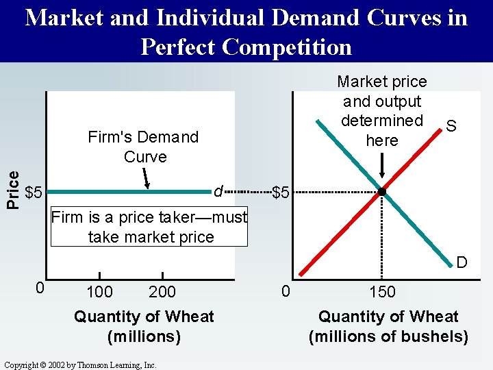
9. 2 The Price Taker’s Demand Curve n Perfectly competitive firms are price takers, selling at the market-determined price. n n An individual seller cannot sell at any price higher than the current market price because buyers could purchase the same good from someone else at the market price. A seller would not charge a lower price when he could sell all he wants at the market price. Copyright © 2002 by Thomson Learning, Inc.

9. 2 The Price Taker’s Demand Curve n n In a perfectly competitive market, an individual seller can change his output and it will not alter the market price. Each producer provides such a small fraction of the total supply that a change in the amount he or she offers does not have a noticeable effect on market price. Copyright © 2002 by Thomson Learning, Inc.

9. 2 The Price Taker’s Demand Curve n n In a perfectly competitive market, then, an individual firm can sell as much as it wishes to place on the market at the prevailing price. In other words, the demand, as seen by the seller, is perfectly elastic at the market price. Copyright © 2002 by Thomson Learning, Inc.

9. 2 The Price Taker’s Demand Curve n Since a perfectly competitive seller n n n won't charge more than the market price because no one will buy at higher prices, nor charge less because the seller can sell all she wants at the market price, the demand curve is horizontal at the market price over the entire range of output that she could possibly produce. Copyright © 2002 by Thomson Learning, Inc.

Market and Individual Demand Curves in Perfect Competition Market price and output determined here Price Firm's Demand Curve d $5 S $5 Firm is a price taker—must take market price D 0 100 200 Quantity of Wheat (millions) Copyright © 2002 by Thomson Learning, Inc. 0 150 Quantity of Wheat (millions of bushels)

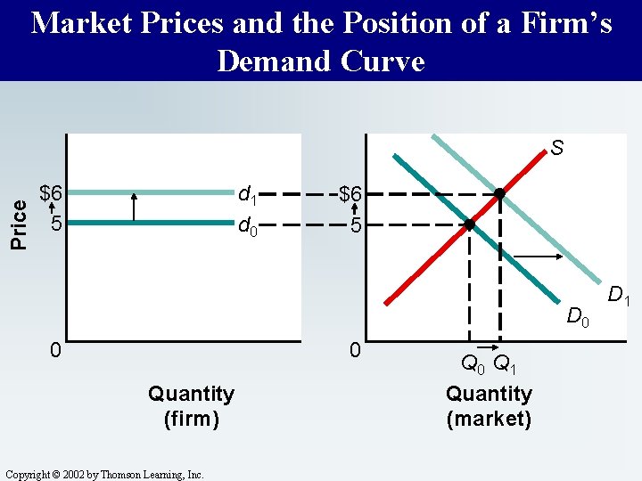
9. 2 The Price Taker’s Demand Curve n n The position or height of each firm’s demand curve varies with every change in the market price. Sellers are provided with current information about market demand supply conditions as a result of price changes. Copyright © 2002 by Thomson Learning, Inc.

9. 2 The Price Taker's Demand Curve n The perfectly competitive model does not assume any knowledge on the part of individual buyers and sellers about market demand supply they only have to know the price of the good they sell. Copyright © 2002 by Thomson Learning, Inc.

Market Prices and the Position of a Firm’s Demand Curve Price S $6 5 d 1 d 0 $6 5 D 0 0 0 Quantity (firm) Copyright © 2002 by Thomson Learning, Inc. Q 0 Q 1 Quantity (market) D 1

9. 3 Profit Maximization n n The firm’s objective is to maximize profits. It wants to produce the amount that maximizes the difference between its total revenues and total costs. Copyright © 2002 by Thomson Learning, Inc.

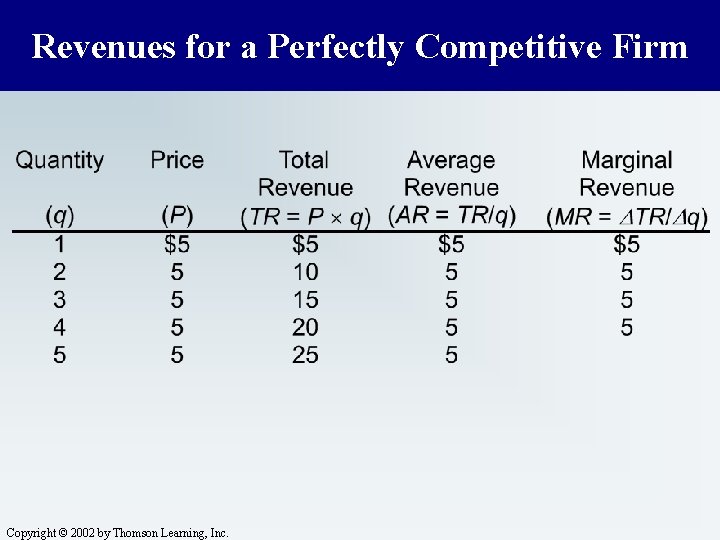
9. 3 Profit Maximization n n Total revenue (TR) is the revenue that the firm receives from the sale of its products. Total revenue for a perfectly competitive firm equals the market price of the good (P) times the quantity (q) of units sold: (TR = P x q). Copyright © 2002 by Thomson Learning, Inc.

9. 3 Profit Maximization n Average revenue (AR) equals total revenue divided by the number of units sold of the product (TR/q). Copyright © 2002 by Thomson Learning, Inc.

9. 3 Profit Maximization n n Marginal revenue (MR) is the additional revenue derived from the sale of one more unit of the good. In a perfectly competitive market, n n additional units of output can be sold without reducing the market price, therefore marginal revenue is constant and equal to the market price, which is also the average revenue. Copyright © 2002 by Thomson Learning, Inc.

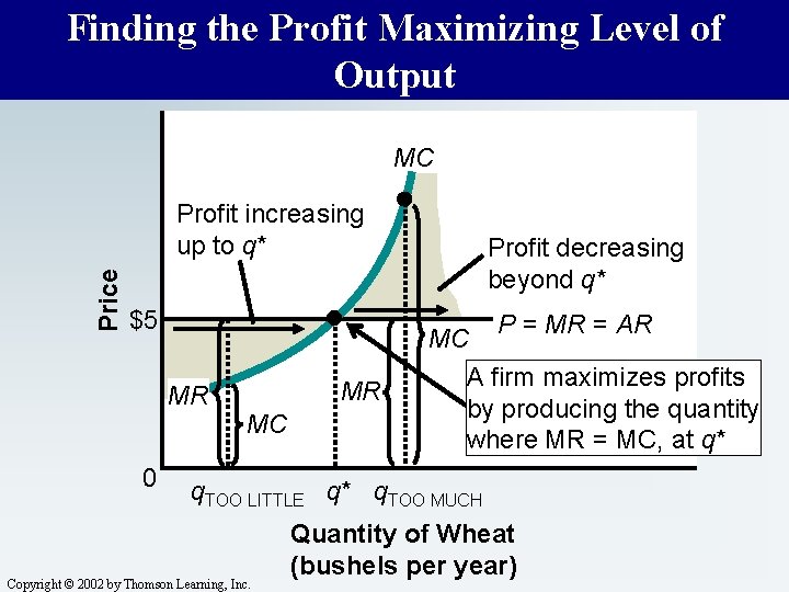
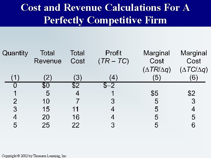
9. 3 Profit Maximization n n In perfect competition, marginal revenue, average revenue, and price are all equal: P = MR = AR. There are two methods for identifying a firm's profit maximizing output. n n the marginal approach the total cost-total revenue approach Copyright © 2002 by Thomson Learning, Inc.

Revenues for a Perfectly Competitive Firm Copyright © 2002 by Thomson Learning, Inc.

9. 3 Profit Maximization n In all types of market environments, firms will maximize profits at that output where one maximizes the difference between total revenue and total costs, which is the same output level where marginal revenue equals marginal costs. Copyright © 2002 by Thomson Learning, Inc.

9. 3 Profit Maximization n The importance of equating marginal revenue and marginal costs for maximizing profits is straightforward. Copyright © 2002 by Thomson Learning, Inc.

9. 3 Profit Maximization n n As long as the marginal revenue derived from expanded output exceeds the marginal cost of that output, the expansion of output creates additional profits. However, expansion of output when the marginal cost of production exceeds marginal revenue will lead to losses on the additional output, decreasing profits. Copyright © 2002 by Thomson Learning, Inc.

9. 3 Profit Maximization n The profit-maximizing output rule says a firm should always produce where its MR = MC. Copyright © 2002 by Thomson Learning, Inc.

Finding the Profit Maximizing Level of Output MC Price Profit increasing up to q* $5 MR 0 MR MC Profit decreasing beyond q* P = MR = AR MC A firm maximizes profits by producing the quantity where MR = MC, at q* q. TOO LITTLE q* q. TOO MUCH Copyright © 2002 by Thomson Learning, Inc. Quantity of Wheat (bushels per year)

9. 3 Profit Maximization n Total revenues and total costs and the profit-maximizing output rule give the same result. Copyright © 2002 by Thomson Learning, Inc.

Cost and Revenue Calculations For A Perfectly Competitive Firm Copyright © 2002 by Thomson Learning, Inc.

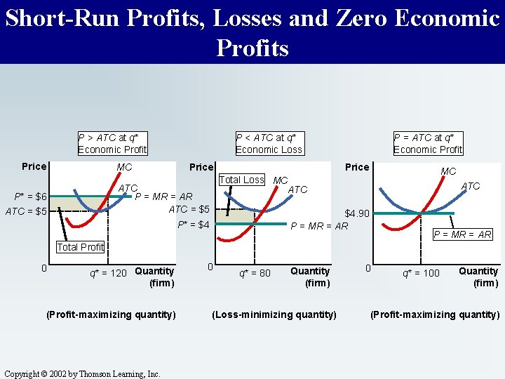
9. 4 Short-Run Profits and Losses n Producing at the profit-maximizing output level does not mean that a firm is actually generating profits. n n It merely means that a firm is maximizing its profit opportunity at a given price level. A firm could be earning profits, n generating losses, or n breaking even. n Copyright © 2002 by Thomson Learning, Inc.

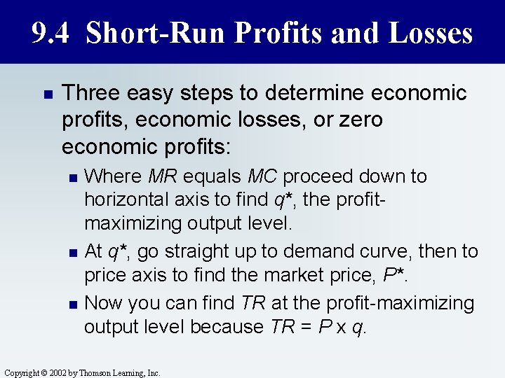
9. 4 Short-Run Profits and Losses n Three easy steps to determine economic profits, economic losses, or zero economic profits: n n n Where MR equals MC proceed down to horizontal axis to find q*, the profitmaximizing output level. At q*, go straight up to demand curve, then to price axis to find the market price, P*. Now you can find TR at the profit-maximizing output level because TR = P x q. Copyright © 2002 by Thomson Learning, Inc.

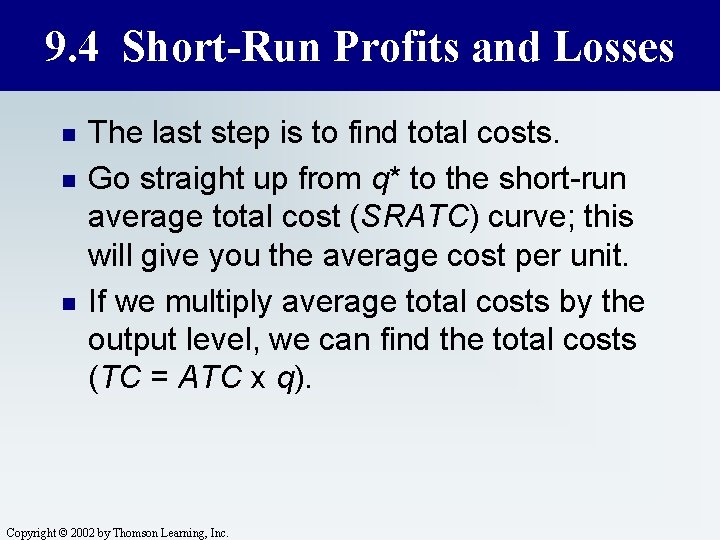
9. 4 Short-Run Profits and Losses n n n The last step is to find total costs. Go straight up from q* to the short-run average total cost (SRATC) curve; this will give you the average cost per unit. If we multiply average total costs by the output level, we can find the total costs (TC = ATC x q). Copyright © 2002 by Thomson Learning, Inc.

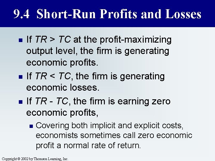
9. 4 Short-Run Profits and Losses n n n If TR > TC at the profit-maximizing output level, the firm is generating economic profits. If TR < TC, the firm is generating economic losses. If TR - TC, the firm is earning zero economic profits, n Covering both implicit and explicit costs, economists sometimes call zero economic profit a normal rate of return. Copyright © 2002 by Thomson Learning, Inc.

Short-Run Profits, Losses and Zero Economic Profits P > ATC at q* Economic Profit Price MC P < ATC at q* Economic Loss Price MC Total Loss MC ATC P = MR = AR ATC = $5 P* = $6 ATC = $5 P = ATC at q* Economic Profit ATC $4. 90 P = MR = AR P* = $4 P = MR = AR Total Profit 0 q* = 120 Quantity (firm) (Profit-maximizing quantity) Copyright © 2002 by Thomson Learning, Inc. 0 q* = 80 Quantity (firm) (Loss-minimizing quantity) 0 q* = 100 Quantity (firm) (Profit-maximizing quantity)

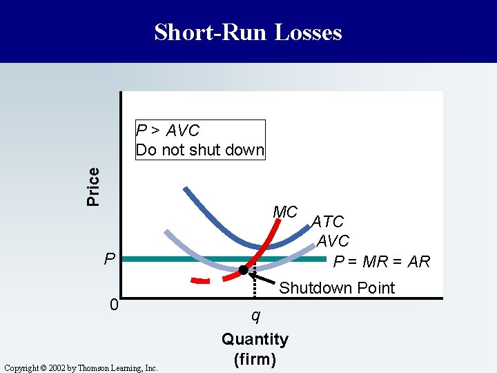
9. 4 Short-Run Profits and Losses n A firm generating an economic loss faces a tough choice: n n n Should it continue to produce or shut-down its operation? To make this decision, we need to consider average variable costs. Copyright © 2002 by Thomson Learning, Inc.

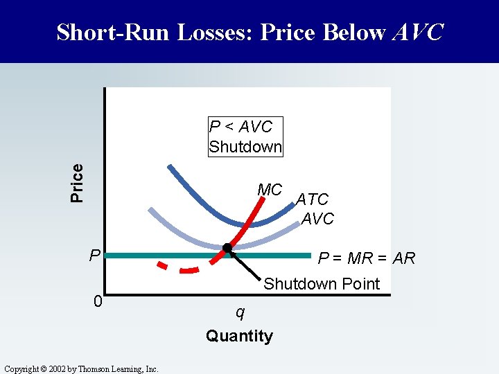
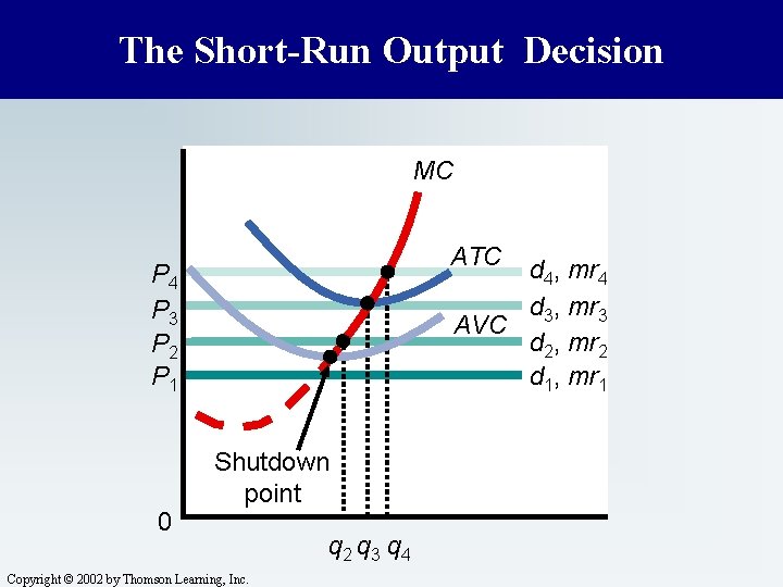
9. 4 Short-Run Profits and Losses n If a firm cannot generate enough revenues to cover its variable costs, then it will have larger losses if it operates than if it shuts down n n (losses in that case = fixed costs). Thus, a firm will not produce at all unless the price is greater than its average variable costs. Copyright © 2002 by Thomson Learning, Inc.

9. 4 Short-Run Profits and Losses n At price levels greater than or equal to average variable costs, a firm may continue to operate in the short run even if average total costs variable and fixed costs are not completely covered. n Because fixed costs continue whether the firm produces or not, it is better to earn enough to cover a portion of these costs rather than earn nothing at all. Copyright © 2002 by Thomson Learning, Inc.

9. 4 Short-Run Profits and Losses n When price is less than average total costs but more than average variable costs, the firm produces in the short run, but at a loss. n To shut down would make this firm worse off because it can cover at least some of its fixed costs with the excess of revenue over its variable costs. Copyright © 2002 by Thomson Learning, Inc.

Short-Run Losses Price P > AVC Do not shut down MC P 0 Copyright © 2002 by Thomson Learning, Inc. ATC AVC P = MR = AR Shutdown Point q Quantity (firm)

9. 4 Short-Run Profits and Losses n When the price a firm is able to obtain for its product is below its average variable costs at all ranges of output, it is unable to cover even its variable costs in the short run. n Since it is losing even more than the fixed costs it would lose if it shut down, it is most logical for the firm to cease operations. Copyright © 2002 by Thomson Learning, Inc.

Short-Run Losses: Price Below AVC Price P < AVC Shutdown MC P 0 Copyright © 2002 by Thomson Learning, Inc. ATC AVC P = MR = AR Shutdown Point q Quantity

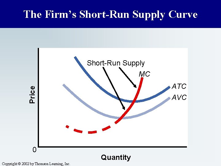
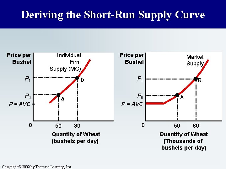
9. 4 Short-Run Profits and Losses n n n At all prices above minimum AVC, the firm produces in the short run, even if ATC is not completely covered. At all prices below the minimum AVC the firm shuts down. Therefore the short-run supply curve of an individual competitive seller is identical with that portion of the MC curve that lies above the minimum of the AVC curve. Copyright © 2002 by Thomson Learning, Inc.

9. 4 Short-Run Profits and Losses n n As a cost relation, the MC curve above minimum AVC shows the marginal cost of producing any given output. As a supply curve, the MC curve above minimum AVC shows the equilibrium output that the firm will supply at various prices in the short run. Copyright © 2002 by Thomson Learning, Inc.

9. 4 Short-Run Profits and Losses n Beyond the point of lowest AVC, the MC of successively larger outputs are progressively greater, so the firm will supply larger amounts only at higher prices. Copyright © 2002 by Thomson Learning, Inc.

The Firm’s Short-Run Supply Curve Short-Run Supply MC Price ATC AVC 0 Copyright © 2002 by Thomson Learning, Inc. Quantity

9. 4 Short-Run Profits and Losses n The short-run market supply curve n n n is the horizontal summation of the individual firms' supply curves, providing that input prices are not affected by increased production of existing firms. Because the short run is too brief for new firms to enter the market, the market supply curve is the horizontal summation of existing firms. Copyright © 2002 by Thomson Learning, Inc.

Deriving the Short-Run Supply Curve Price per Bushel Individual Firm Supply (MC) P 1 P 0 P = AVC 0 b 80 Quantity of Wheat (bushels per day) Copyright © 2002 by Thomson Learning, Inc. Market Supply P 1 P 0 P = AVC a 50 Price per Bushel 0 B B A A 50 80 Quantity of Wheat (Thousands of bushels per day)

The Short-Run Output Decision MC ATC d 4, mr 4 d 3, mr 3 AVC d 2, mr 2 d 1, mr 1 P 4 P 3 P 2 P 1 0 Shutdown point Copyright © 2002 by Thomson Learning, Inc. q 2 q 3 q 4

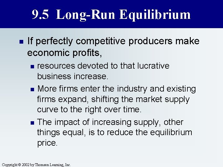
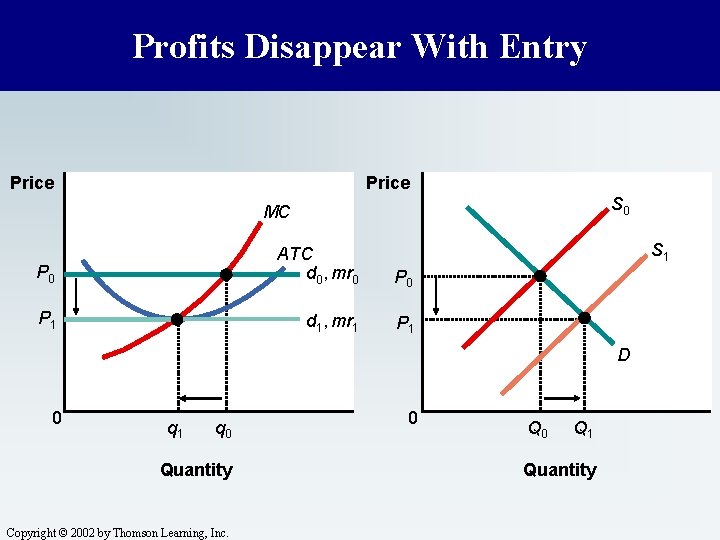
9. 5 Long-Run Equilibrium n If perfectly competitive producers make economic profits, n n n resources devoted to that lucrative business increase. More firms enter the industry and existing firms expand, shifting the market supply curve to the right over time. The impact of increasing supply, other things equal, is to reduce the equilibrium price. Copyright © 2002 by Thomson Learning, Inc.

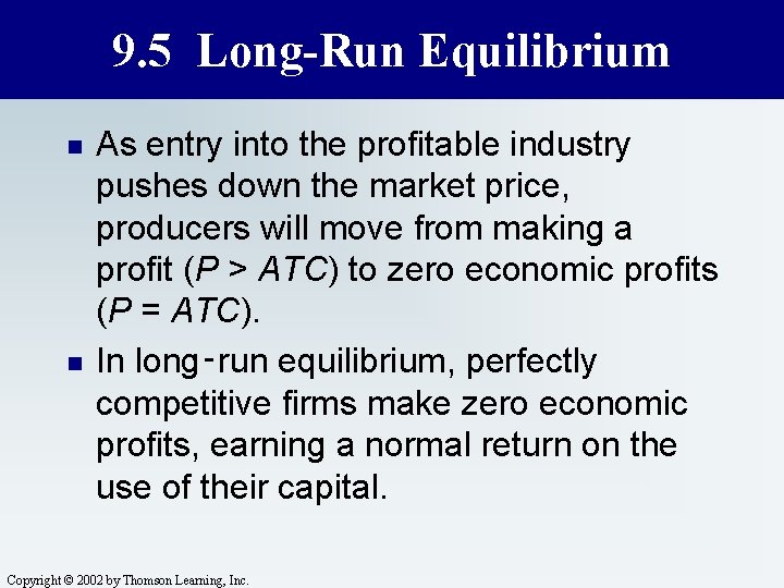
9. 5 Long-Run Equilibrium n n As entry into the profitable industry pushes down the market price, producers will move from making a profit (P > ATC) to zero economic profits (P = ATC). In long‑run equilibrium, perfectly competitive firms make zero economic profits, earning a normal return on the use of their capital. Copyright © 2002 by Thomson Learning, Inc.

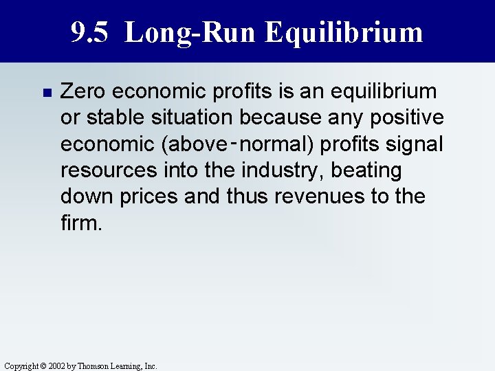
9. 5 Long-Run Equilibrium n Zero economic profits is an equilibrium or stable situation because any positive economic (above‑normal) profits signal resources into the industry, beating down prices and thus revenues to the firm. Copyright © 2002 by Thomson Learning, Inc.

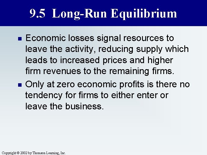
9. 5 Long-Run Equilibrium n n Economic losses signal resources to leave the activity, reducing supply which leads to increased prices and higher firm revenues to the remaining firms. Only at zero economic profits is there no tendency for firms to either enter or leave the business. Copyright © 2002 by Thomson Learning, Inc.

Profits Disappear With Entry Price S 0 MC S 1 P 0 ATC d 0, mr 0 P 1 d 1, mr 1 P 1 D 0 q 1 q 0 Quantity Copyright © 2002 by Thomson Learning, Inc. 0 Q 1 Quantity

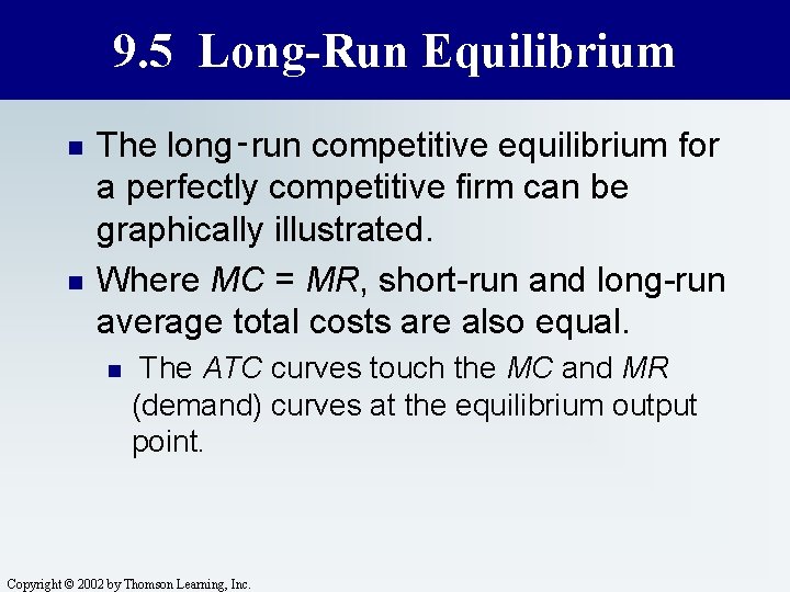
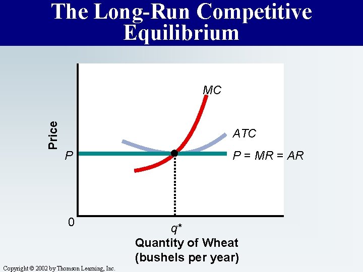
9. 5 Long-Run Equilibrium n n The long‑run competitive equilibrium for a perfectly competitive firm can be graphically illustrated. Where MC = MR, short-run and long-run average total costs are also equal. n The ATC curves touch the MC and MR (demand) curves at the equilibrium output point. Copyright © 2002 by Thomson Learning, Inc.

9. 5 Long-Run Equilibrium n Because the MR curve is also the AR curve, average revenues and average total costs are equal at the equilibrium point. Copyright © 2002 by Thomson Learning, Inc.

9. 5 Long-Run Equilibrium n The long-run equilibrium output in perfect competition occurs at the lowest point on the ATC curve, so the equilibrium condition in the long run in perfect competition is for firms to produce at that output that minimizes per-unit total costs. Copyright © 2002 by Thomson Learning, Inc.

The Long-Run Competitive Equilibrium Price MC ATC P 0 Copyright © 2002 by Thomson Learning, Inc. P = MR = AR q* Quantity of Wheat (bushels per year)

9. 6 Long-Run Supply n When the output of an entire industry changes, we consider two possible industry cost conditions. n n n constant costs increasing costs The shape of the long-run supply curve depends on the extent to which input costs change when there is entry or exit of firms in the industry. Copyright © 2002 by Thomson Learning, Inc.

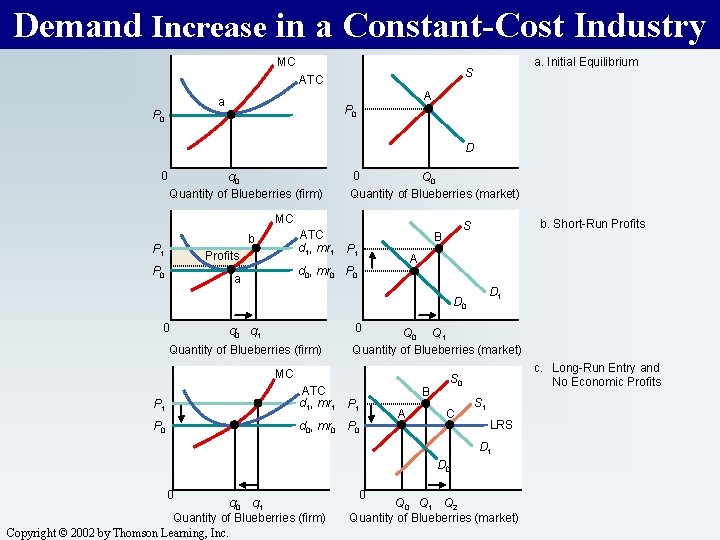
9. 6 Long-Run Supply n In a constant-cost industry, the prices of inputs do not change as output is expanded. The industry does not use inputs in sufficient quantities to affect input prices. Copyright © 2002 by Thomson Learning, Inc.

9. 6 Long-Run Supply n Because the industry is one of constant costs, industry expansion does not alter firm's cost curves, and the industry longrun supply curve is horizontal. Copyright © 2002 by Thomson Learning, Inc.

9. 6 Long-Run Supply n n n The short-run higher profits from an increase in demand attracts entry until long-run equilibrium is again reached. The long‑run equilibrium price is at the same level that prevailed before demand increased. The only long‑run effect of the increase in demand is an increase in industry output. Copyright © 2002 by Thomson Learning, Inc.

Demand Increase in a Constant-Cost Industry MC ATC A a P 0 a. Initial Equilibrium S P 0 D 0 q 0 Quantity of Blueberries (firm) 0 Quantity of Blueberries (market) MC ATC d 1, mr 1 P 1 b P 1 Profits P 0 B A d 0, mr 0 P 0 a b. Short-Run Profits S D 1 D 0 0 0 q 1 Quantity of Blueberries (firm) Q 0 Q 1 Quantity of Blueberries (market) MC P 1 ATC d 1, mr 1 P 0 d 0, mr 0 P 0 B A c. Long-Run Entry and No Economic Profits S 0 C S 1 LRS D 1 D 0 0 q 1 Quantity of Blueberries (firm) Copyright © 2002 by Thomson Learning, Inc. 0 Q 1 Q 2 Quantity of Blueberries (market)

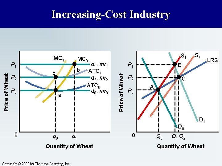
9. 6 Long-Run Supply n In an increasing-cost industry, the cost curves of the individual firms rise as the total output of the industry increases. Copyright © 2002 by Thomson Learning, Inc.

9. 6 Long-Run Supply n When an industry utilizes a large portion of an input, n n n input prices will rise when the industry uses more of that input as it expands output, which will shift firms' cost curves upward. Examples include “extractive” industries, which utilize large portions of the total supply of specialized natural resources such as land or mineral deposits. Copyright © 2002 by Thomson Learning, Inc.

9. 6 Long-Run Supply n n The short-run higher profits from an increase in demand attracts entry until long-run equilibrium is again reached; producers' MC and AC curves will be higher, so that the new long-run equilibrium is at a higher price. The long-run industry supply curve in this case has a positive slope. Copyright © 2002 by Thomson Learning, Inc.

Increasing-Cost Industry P 2 b c P 0 S 1 MC 0 a d 1, mr 1 ATC 1 d 2, mr 2 ATC 0 d 0, mr 0 P 1 Price of Wheat P 1 MC 1 B P 2 P 0 C A D 0 0 q 1 Quantity of Wheat Copyright © 2002 by Thomson Learning, Inc. 0 S 1 Q 0 D 1 Q 2 Quantity of Wheat LRS

9. 6 Long-Run Supply n Even in this case, the long-run supply is usually more elastic than the short-run supply because in the long run, firms can enter and exit the industry. Copyright © 2002 by Thomson Learning, Inc.

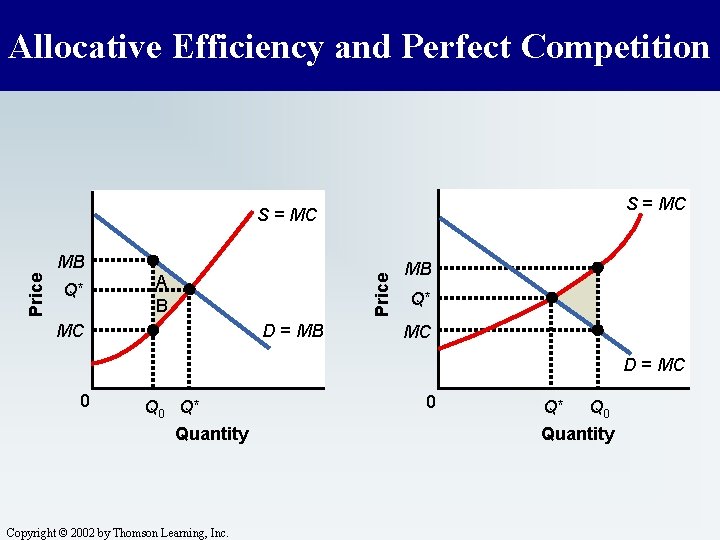
9. 6 Long-Run Supply n n The output that results from equilibrium conditions of market demand supply in perfectly competitive markets is economically efficient. Only at this outcome can maximum output be obtained from our scarce resources. Copyright © 2002 by Thomson Learning, Inc.

9. 6 Long-Run Supply n Once the competitive equilibrium is reached, n n n the buyers' marginal benefit equal the sellers' marginal cost (both equal to the price) and the sum of consumer and producer surplus is maximized. If there are no externalities, then total welfare is maximized and resources are allocated efficiently. Copyright © 2002 by Thomson Learning, Inc.

Allocative Efficiency and Perfect Competition S = MC Q* A B Price MB D = MB MC MB Q* MC D = MC 0 Q* Quantity Copyright © 2002 by Thomson Learning, Inc. 0 Q* Q 0 Quantity