A Lecture Presentation in Power Point to accompany

A Lecture Presentation in Power. Point to accompany Essentials of Economics by Robert L. Sexton Copyright © 2003 Thomson Learning, Inc. Thomson Learning™ is a trademark used herein under license. ALL RIGHTS RESERVED. Instructors of classes adopting EXPLORING ECONOMICS, Second Edition by Robert L. Sexton as an assigned textbook may reproduce material from this publication for classroom use or in a secure electronic network environment that prevents downloading or reproducing the copyrighted material. Otherwise, no part of this work covered by the copyright hereon may be reproduced or used in any form or by any means—graphic, electronic, or mechanical, including, but not limited to, photocopying, recording, taping, Web distribution, information networks, or information storage and retrieval systems—without the written permission of the publisher. Printed in the United States of America ISBN 0030342333 Copyright © 2003 by Thomson Learning, Inc.

Chapter 15 Aggregate Supply and Macroeconomic Equilibrium Copyright © 2003 by Thomson Learning, Inc.

15. 1 The Aggregate Supply Curve n n The Aggregate supply (AS) curve is the relationship between the total quantity of final goods and services that suppliers are willing and able to produce and the overall price level. The aggregate supply curve represents how much RGDP suppliers will be willing to produce at different price levels. Copyright © 2003 by Thomson Learning, Inc.

15. 1 The Aggregate Supply Curve n In fact, there are two aggregate supply curves. n Short-run aggregate supply (SRAS) n n a period when output can change in response to supply and demand, but input prices have not yet been able to adjust Long-run aggregate supply (LRAS) n a period long enough for the prices of outputs and all inputs to fully adjust to changes in the economy Copyright © 2003 by Thomson Learning, Inc.

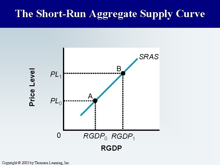
15. 1 The Aggregate Supply Curve n In the short run, the aggregate supply curve is upward sloping. n n At higher price levels, producers are willing to supply more real output. At lower price levels, they are willing to supply less real output. Copyright © 2003 by Thomson Learning, Inc.

The Short-Run Aggregate Supply Curve Price Level SRAS B PL 1 PL 0 0 A RGDP 0 RGDP 1 RGDP Copyright © 2003 by Thomson Learning, Inc.

15. 1 The Aggregate Supply Curve n n Why would producers be willing to supply more output just because the price level increases? There are two possible explanations. n n profit effect misperception effect Copyright © 2003 by Thomson Learning, Inc.

15. 1 The Aggregate Supply Curve n n n To many firms, input costs like wages and rents are relatively constant in the short run. The slow adjustments of input prices are due to the longer-term input contracts that do not adjust quickly to price changes. So when the price level rises, output prices rise relative to input prices (costs), raising producers’ short-run profit margins. Copyright © 2003 by Thomson Learning, Inc.

15. 1 The Aggregate Supply Curve n n n These increased profit margins make it in the producers’ self-interest to expand their production and sales at higher price levels. If the price level falls, output prices fall and producers’ profits tend to fall. When output prices fall, producers will find it more difficult to cover their input costs, and consequently, will reduce their level of output. Copyright © 2003 by Thomson Learning, Inc.

15. 1 The Aggregate Supply Curve n n The second explanation of the upwardsloping short-run aggregate supply curve is that producers can be fooled by price changes in the short run. If a producer sees the price of his output rising and thinks that the relative price of his output is rising (i. e. , that his product is becoming more valuable in real terms), he will supply more. Copyright © 2003 by Thomson Learning, Inc.

15. 1 The Aggregate Supply Curve n n n It might be that it was not just his goods prices that were rising; the prices of many other goods and services could also be rising at the same time as a result of an increase in the price level. The relative price of his output, then, was not actually rising, although it appeared so in the short run. In this case, the producer was fooled into supplying more based on his shortrun misperception of relative prices. Copyright © 2003 by Thomson Learning, Inc.

15. 1 The Aggregate Supply Curve n n Along the short-run aggregate supply curve, we assume that wages and other input prices are constant. This is not the case in the long run, which is a period long enough for the price of all inputs to fully adjust to changes in the economy. Copyright © 2003 by Thomson Learning, Inc.

15. 1 The Aggregate Supply Curve n Along the long-run aggregate supply curve, we are looking at the relationship between RGDP produced and the price level, once input prices have been able to respond to changes in output prices. Copyright © 2003 by Thomson Learning, Inc.

15. 1 The Aggregate Supply Curve n n Along the LRAS curve, two sets of prices are changing the prices of outputs and the price of inputs. Along the LRAS curve, a 10 percent increase in the price of goods and services is matched by a 10 percent increase in the price of inputs. Copyright © 2003 by Thomson Learning, Inc.

15. 1 The Aggregate Supply Curve n The long-run aggregate supply curve is insensitive to the price level, reflecting the fact that the level of RGDP producers are willing to supply is not affected by changes in the price level. Copyright © 2003 by Thomson Learning, Inc.

15. 1 The Aggregate Supply Curve n n The vertical LRAS curve will always be positioned at the natural rate of output, where all resources are fully employed. In the long run, firms will always produce at the maximum sustainable level allowed by their capital, labor, and technological inputs, regardless of the price level. Copyright © 2003 by Thomson Learning, Inc.

15. 1 The Aggregate Supply Curve n The long-run equilibrium level is where the economy will settle when undisturbed, and all resources are fully employed. Copyright © 2003 by Thomson Learning, Inc.

15. 1 The Aggregate Supply Curve n n The economy will always be at the intersection of AS and AD but that will not always be at the natural rate of output. Long-run equilibrium will only occur where AS and AD intersect along the long-run aggregate supply curve at the natural, or potential, rate of output. Copyright © 2003 by Thomson Learning, Inc.

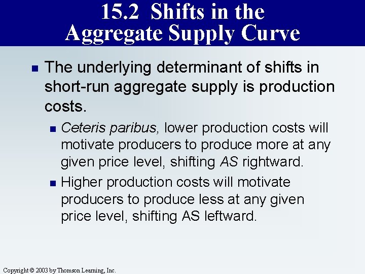
15. 2 Shifts in the Aggregate Supply Curve n The underlying determinant of shifts in short-run aggregate supply is production costs. n n Ceteris paribus, lower production costs will motivate producers to produce more at any given price level, shifting AS rightward. Higher production costs will motivate producers to produce less at any given price level, shifting AS leftward. Copyright © 2003 by Thomson Learning, Inc.

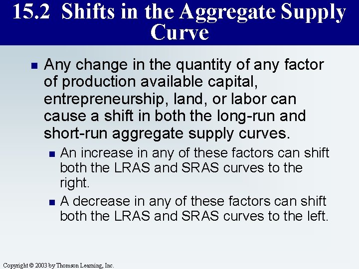
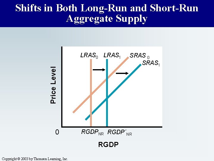
15. 2 Shifts in the Aggregate Supply Curve n Any change in the quantity of any factor of production available capital, entrepreneurship, land, or labor can cause a shift in both the long-run and short-run aggregate supply curves. n n An increase in any of these factors can shift both the LRAS and SRAS curves to the right. A decrease in any of these factors can shift both the LRAS and SRAS curves to the left. Copyright © 2003 by Thomson Learning, Inc.

Shifts in Both Long-Run and Short-Run Aggregate Supply Price Level LRAS 0 LRAS 1 0 RGDPNR RGDP´NR RGDP Copyright © 2003 by Thomson Learning, Inc. SRAS 0 SRAS 1

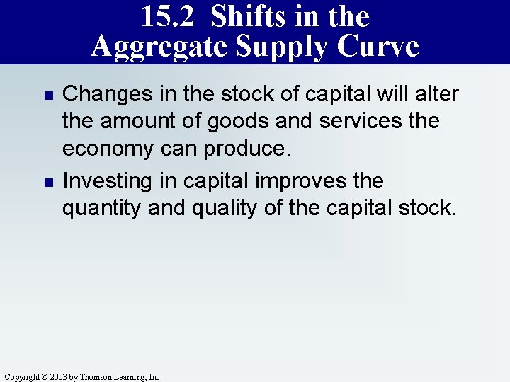
15. 2 Shifts in the Aggregate Supply Curve n n Changes in the stock of capital will alter the amount of goods and services the economy can produce. Investing in capital improves the quantity and quality of the capital stock. Copyright © 2003 by Thomson Learning, Inc.

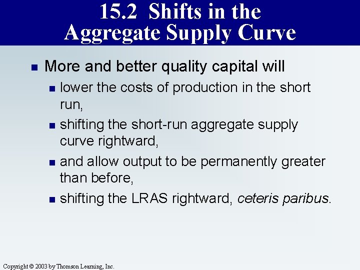
15. 2 Shifts in the Aggregate Supply Curve n More and better quality capital will n n lower the costs of production in the short run, shifting the short-run aggregate supply curve rightward, and allow output to be permanently greater than before, shifting the LRAS rightward, ceteris paribus. Copyright © 2003 by Thomson Learning, Inc.

15. 2 Shifts in the Aggregate Supply Curve n n n Changes in human capital can also alter the aggregate supply curve. Investments in human capital may include educational or vocational programs or on-the-job training. All of these investments in human capital would cause productivity to rise. Copyright © 2003 by Thomson Learning, Inc.

15. 2 Shifts in the Aggregate Supply Curve n As a result, the short-run aggregate supply curve would shift to the right because a more skilled workforce will lower the costs of production, and the LRAS curve would shift to the right because greater output is achievable on a permanent, or sustainable, basis, ceteris paribus. Copyright © 2003 by Thomson Learning, Inc.

15. 2 Shifts in the Aggregate Supply Curve n n Through their inventive activity, entrepreneurs lower costs and expand real output possibilities. If entrepreneurial activities lower the costs of production and expand what can be produced with the resources available to the economy, then the short -run and long-run aggregate supply curves both shift to the right. Copyright © 2003 by Thomson Learning, Inc.

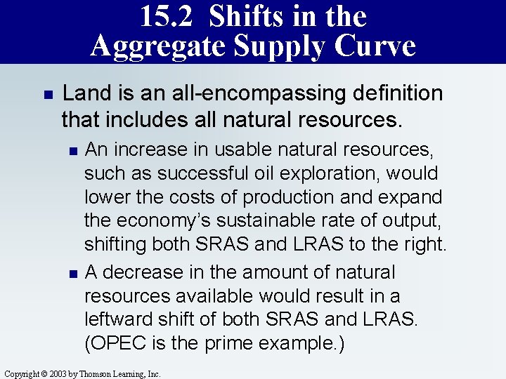
15. 2 Shifts in the Aggregate Supply Curve n Land is an all-encompassing definition that includes all natural resources. n n An increase in usable natural resources, such as successful oil exploration, would lower the costs of production and expand the economy’s sustainable rate of output, shifting both SRAS and LRAS to the right. A decrease in the amount of natural resources available would result in a leftward shift of both SRAS and LRAS. (OPEC is the prime example. ) Copyright © 2003 by Thomson Learning, Inc.

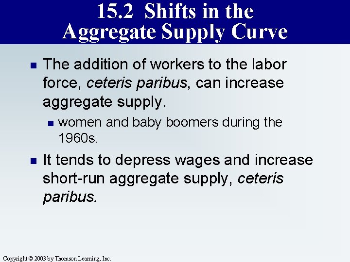
15. 2 Shifts in the Aggregate Supply Curve n The addition of workers to the labor force, ceteris paribus, can increase aggregate supply. n n women and baby boomers during the 1960 s. It tends to depress wages and increase short-run aggregate supply, ceteris paribus. Copyright © 2003 by Thomson Learning, Inc.

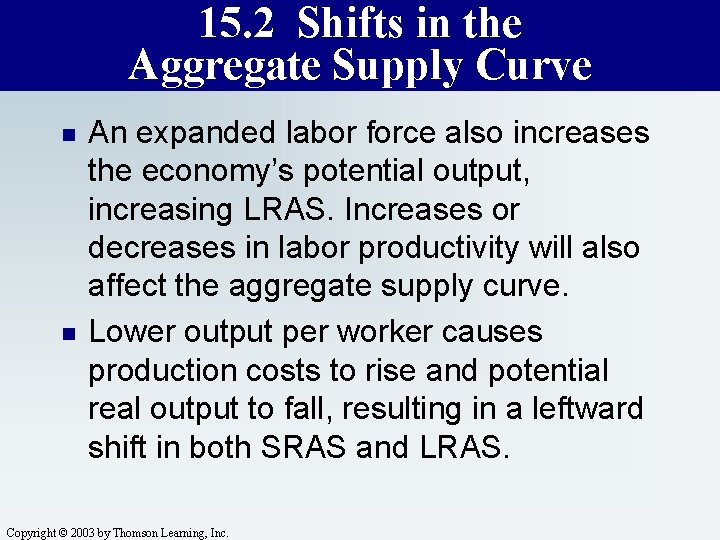
15. 2 Shifts in the Aggregate Supply Curve n n An expanded labor force also increases the economy’s potential output, increasing LRAS. Increases or decreases in labor productivity will also affect the aggregate supply curve. Lower output per worker causes production costs to rise and potential real output to fall, resulting in a leftward shift in both SRAS and LRAS. Copyright © 2003 by Thomson Learning, Inc.

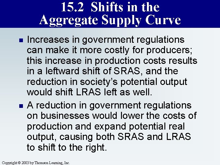
15. 2 Shifts in the Aggregate Supply Curve n n Increases in government regulations can make it more costly for producers; this increase in production costs results in a leftward shift of SRAS, and the reduction in society’s potential output would shift LRAS left as well. A reduction in government regulations on businesses would lower the costs of production and expand potential real output, causing both SRAS and LRAS to shift to the right. Copyright © 2003 by Thomson Learning, Inc.

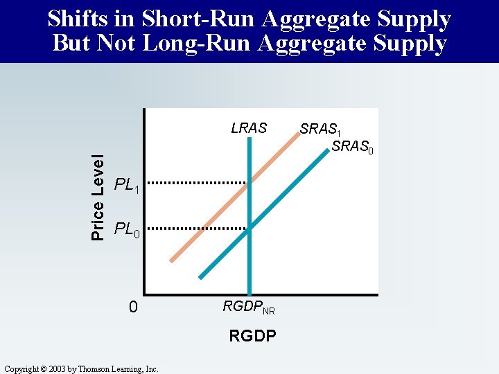
15. 2 Shifts in the Aggregate Supply Curve n n Some factors shift SRAS but do not impact LRAS. The most important of these factors are changes in input prices and natural disasters. n The price of factors, or inputs, that go into producing outputs will affect only SRAS if they don’t reflect permanent changes in the suppliers of some factors of production. Copyright © 2003 by Thomson Learning, Inc.

Shifts in Short-Run Aggregate Supply But Not Long-Run Aggregate Supply Price Level LRAS PL 1 PL 0 0 RGDPNR RGDP Copyright © 2003 by Thomson Learning, Inc. SRAS 1 SRAS 0

15. 2 Shifts in the Aggregate Supply Curve n n If wages increase without a corresponding increase in labor productivity, then it will become more costly for suppliers to produce goods and services at every price level, causing SRAS to shift to the left. LRAS will not shift because with the same supply of labor as before, potential output does not change. Copyright © 2003 by Thomson Learning, Inc.

15. 2 Shifts in the Aggregate Supply Curve n n If the price of steel rises, automobile producers will find it more expensive to do business because their production costs will rise, again resulting in a leftward shift in SRAS. The LRAS will not shift as long as the capacity to make steel has not been reduced. Copyright © 2003 by Thomson Learning, Inc.

15. 2 Shifts in the Aggregate Supply Curve n n It is supply and demand in factor markets (like capital, land, and labor) that cause input prices to change. The reason that changes in input prices only affect SRAS and not LRAS, unless they reflect permanent changes in the supplies of those inputs, lies in our definition of long-run aggregate supply. Copyright © 2003 by Thomson Learning, Inc.

15. 2 Shifts in the Aggregate Supply Curve n n The LRAS is vertical at the natural level of real output, determined by the supplies of the various factors of production. A fall in input prices, which shifts SRAS right, only shifts LRAS right if potential output has risen, and this only occurs if the supply of those inputs is increased. Copyright © 2003 by Thomson Learning, Inc.

15. 2 Shifts in the Aggregate Supply Curve n n n Adverse supply shocks, such as natural disasters, can increase the costs of production. They could cause SRAS to shift to the left, ceteris paribus. However, once the temporary effects of these disasters have been felt, no appreciable change in the economy’s productive capacity has occurred, so LRAS doesn’t shift as a result. Copyright © 2003 by Thomson Learning, Inc.

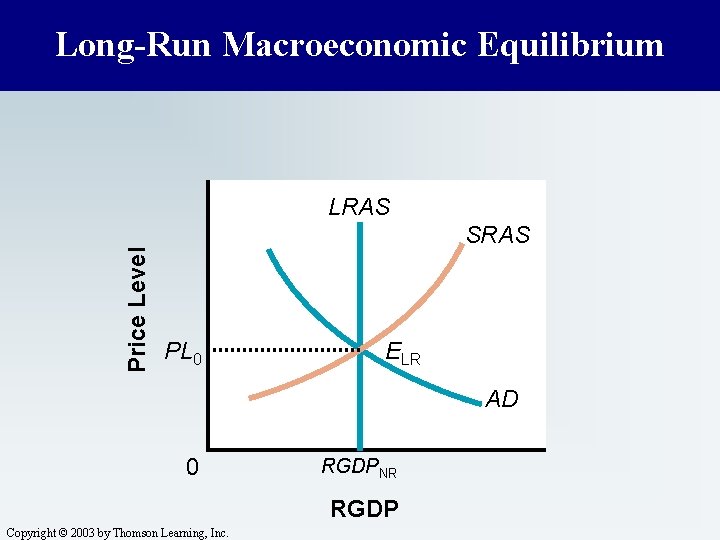
15. 3 Macroeconomic Equilibrium n n The short-run equilibrium level of real output and the price level are determined by the intersection of the aggregate demand curve and the shortrun aggregate supply curve. When this equilibrium occurs at the potential output level, on the long-run aggregate supply curve, the economy is operating at full employment. Copyright © 2003 by Thomson Learning, Inc.

Long-Run Macroeconomic Equilibrium Price Level LRAS SRAS PL 0 ELR AD 0 RGDPNR RGDP Copyright © 2003 by Thomson Learning, Inc.

15. 3 Macroeconomic Equilibrium n n Only a short-run equilibrium that is at potential output is also a long-run equilibrium. Short-run equilibrium can change when n the aggregate demand curve shifts or the short-run aggregate supply curve shifts rightward or leftward, but the long-run equilibrium level of RGDP only changes when the LRAS shifts. Copyright © 2003 by Thomson Learning, Inc.

15. 3 Macroeconomic Equilibrium n Sometimes, these supply or demand changes are anticipated; at other times, however, the shifts occur unexpectedly. Economists call these unexpected shifts shocks. Copyright © 2003 by Thomson Learning, Inc.

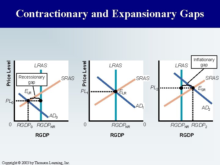
15. 3 Macroeconomic Equilibrium n n Short-run equilibrium can occur at less than the potential output of the economy, resulting in a contractionary gap. Or it can temporarily occur beyond potential output, resulting in an expansionary gap. Copyright © 2003 by Thomson Learning, Inc.

LRAS Recessionary gap SRAS Price Level Contractionary and Expansionary Gaps PL 1 ELR LRAS Inflationary gap SRAS PL 2 ELR PL 0 ESR AD 1 AD 2 AD 0 0 RGDPNR RGDP Copyright © 2003 by Thomson Learning, Inc. 0 RGDPNR RGDP 2 RGDP

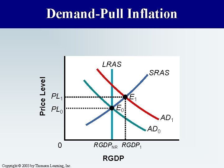
15. 3 Macroeconomic Equilibrium n n n Demand-pull inflation occurs when the price level rises as a result of an increase in aggregate demand. The increase in AD causes an increase in the price level and an increase in real output, illustrated by a movement up along the SRAS curve. This causes an expansionary gap. Copyright © 2003 by Thomson Learning, Inc.

15. 3 Macroeconomic Equilibrium n The increase in output as a result of the increase in the price level is a result of its effect on producers profits; firms have an incentive to increase real output when the prices of the goods they are selling are rising faster than the costs of the inputs they use in production. Copyright © 2003 by Thomson Learning, Inc.

Demand-Pull Inflation Price Level LRAS PL 1 PL 0 SRAS E 1 E 0 AD 1 AD 0 0 RGDPNR RGDP 1 RGDP Copyright © 2003 by Thomson Learning, Inc.

15. 3 Macroeconomic Equilibrium n n The short-run result of an increase in AD is a level of RGDP beyond full employment. The potential output is an expansionary gap. Copyright © 2003 by Thomson Learning, Inc.

15. 3 Macroeconomic Equilibrium n It seems peculiar that the economy can operate beyond its potential, but this is possible, temporarily, as firms n n n encourage workers to work overtime, extend the hours of part time workers, hire recently retired employees, reduce frictional unemployment through more extensive searches for employees, and so on. Copyright © 2003 by Thomson Learning, Inc.

15. 3 Macroeconomic Equilibrium n n Short-run real output beyond potential output (and employment beyond full employment) cannot be sustained in the long run. In the expansionary gap situation, because the price level is now higher, workers (and other input suppliers) become disgruntled with real wages that have not yet adjusted to the new price level. Copyright © 2003 by Thomson Learning, Inc.

15. 3 Macroeconomic Equilibrium n n Recall that along the SRAS curve, wages and other input prices are assumed to be constant. Therefore, workers and input suppliers purchasing power falls as output prices rise. (If prices have risen, but wages have not risen as much, real wages have fallen. ) Because real (adjusted for inflation) wages have fallen, workers and other suppliers demand higher prices in order to supply their inputs. Copyright © 2003 by Thomson Learning, Inc.

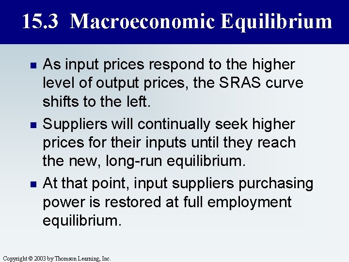
15. 3 Macroeconomic Equilibrium n n n As input prices respond to the higher level of output prices, the SRAS curve shifts to the left. Suppliers will continually seek higher prices for their inputs until they reach the new, long-run equilibrium. At that point, input suppliers purchasing power is restored at full employment equilibrium. Copyright © 2003 by Thomson Learning, Inc.

15. 3 Macroeconomic Equilibrium n n The only long-run difference from the initial equilibrium is the new, higher price level. The 1970 s and early 1980 s witnessed a phenomenon known as stagflation, where lower growth and higher prices occurred together. Copyright © 2003 by Thomson Learning, Inc.

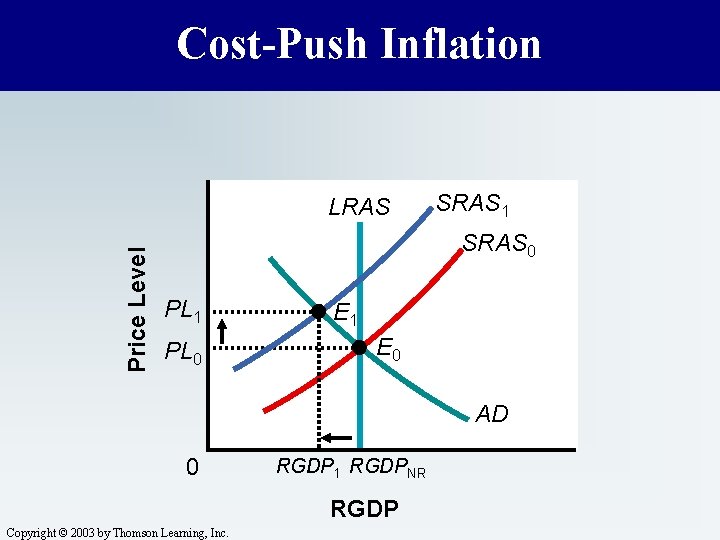
15. 3 Macroeconomic Equilibrium n n Some economists believe that this was caused by a leftward shift in the aggregate supply curve. If aggregate demand did not change significantly and the price level increased, then the inflation was caused by supply-side forces, not demand. This is called cost-push inflation. Copyright © 2003 by Thomson Learning, Inc.

Cost-Push Inflation Price Level LRAS SRAS 1 SRAS 0 PL 1 PL 0 E 1 E 0 AD 0 RGDP 1 RGDPNR RGDP Copyright © 2003 by Thomson Learning, Inc.

15. 3 Macroeconomic Equilibrium n n The primary culprits responsible for the leftward shift in SRAS in the 1970 s were oil price increases. An increase in input prices can cause the SRAS curve to shift to the left, and this spelled big trouble for the U. S. economy: n n n higher price levels, lower output, and higher rates of unemployment. Copyright © 2003 by Thomson Learning, Inc.

15. 3 Macroeconomic Equilibrium n Starting with the economy initially at full employment equilibrium, suppose there is a sudden increase in input prices, such as the increase in the price of oil. Copyright © 2003 by Thomson Learning, Inc.

15. 3 Macroeconomic Equilibrium n n This increase would shift the SRAS curve to the left. As a result, the price level rises and real output falls below potential output. Now firms may demand fewer workers as a result of the higher input costs that cannot be passed on to the consumers. The result is higher prices, lower real output, more unemployment, and a contractionary gap. Copyright © 2003 by Thomson Learning, Inc.

15. 3 Macroeconomic Equilibrium n n n As far as energy prices are concerned, the 1980 s witnessed falling oil prices as OPEC lost some of its clout, and many non-OPEC oil producers increased production. The net result was a rightward shift in the SRAS curve. Holding AD constant, this rightward shift in SRAS would lead to lower prices, greater output, and lower rates of unemployment. Copyright © 2003 by Thomson Learning, Inc.

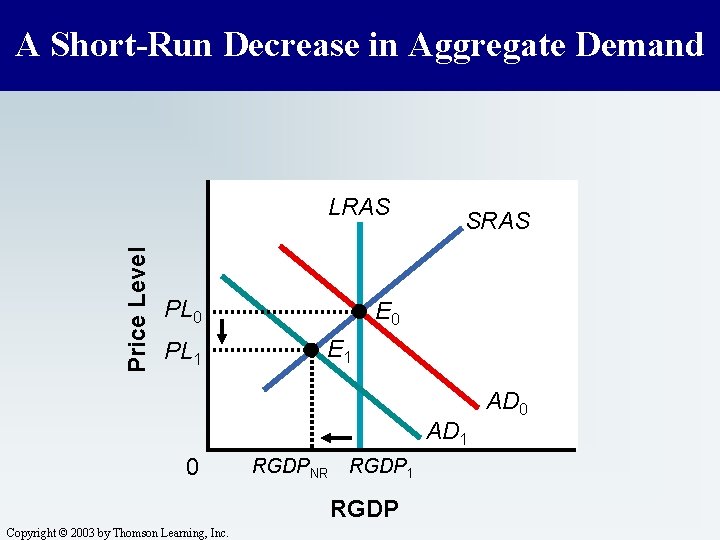
15. 3 Macroeconomic Equilibrium n n Just as cost-push inflation cause a recession, so can a decrease in AD. A fall in AD would reduce real output and the price level, and increase unemployment in the short run—a contractionary gap. Many recoveries from recessions occur because of increases in aggregate demand that take the economy back to potential output. Copyright © 2003 by Thomson Learning, Inc.

A Short-Run Decrease in Aggregate Demand Price Level LRAS PL 0 PL 1 SRAS E 0 E 1 AD 1 0 RGDPNR RGDP 1 RGDP Copyright © 2003 by Thomson Learning, Inc. AD 0

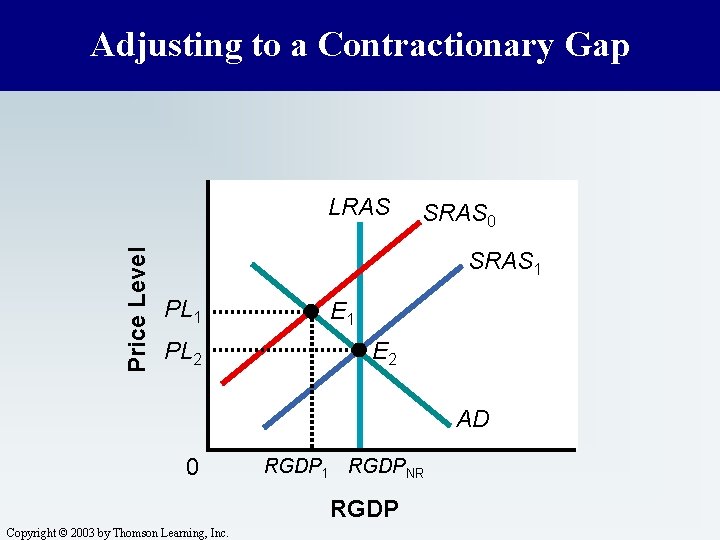
15. 3 Macroeconomic Equilibrium n n It is possible that the economy would self-correct through declining wages and prices. In a recession, unemployed workers and other input suppliers will bid down wages and prices. Copyright © 2003 by Thomson Learning, Inc.

15. 3 Macroeconomic Equilibrium n n The resulting reduction in production costs shifts the short-run aggregate supply curve to the right. Eventually, the economy returns to a long-run equilibrium at potential output and a lower price level. Copyright © 2003 by Thomson Learning, Inc.

Adjusting to a Contractionary Gap Price Level LRAS SRAS 0 SRAS 1 PL 2 E 1 E 2 AD 0 RGDP 1 RGDPNR RGDP Copyright © 2003 by Thomson Learning, Inc.

15. 3 Macroeconomic Equilibrium n n Many economists believe that wages and prices may be very slow to adjust, especially downward. This downward wage stickiness may lead to prolonged periods of recession, by making the economy’s adjustment mechanism slower. Copyright © 2003 by Thomson Learning, Inc.

15. 3 Macroeconomic Equilibrium n Wages and prices may be sticky downward because of n n long-term labor contracts, a legal minimum wage, employers paying efficiency wages, and menu costs. Copyright © 2003 by Thomson Learning, Inc.

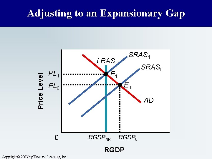
15. 3 Macroeconomic Equilibrium n If the economy is currently in an expansionary gap, with output greater than potential output, the price level is higher than workers anticipated, and workers’ and input suppliers’ purchasing power has fallen. Copyright © 2003 by Thomson Learning, Inc.

15. 3 Macroeconomic Equilibrium n Consequently, workers and other suppliers demand higher prices to be willing to supply their inputs, shifting the short-run aggregate supply to the left, until they reach the long-run equilibrium at potential output. Input suppliers’ purchasing power is restored at a higher price level. Copyright © 2003 by Thomson Learning, Inc.

Adjusting to an Expansionary Gap SRAS 1 Price Level LRAS PL 1 SRAS 0 E 1 E 0 PL 0 AD 0 RGDPNR RGDP 0 RGDP Copyright © 2003 by Thomson Learning, Inc.

15. 3 Macroeconomic Equilibrium n n In this chapter, we have been shifting the AS and AD curves around as if we knew exactly what we were doing. But it is very important to mention that the AD/AS model is a crude tool. Copyright © 2003 by Thomson Learning, Inc.

15. 3 Macroeconomic Equilibrium n n In the supply and demand curves covered in Chapter 4, we saw how this simple tool is very rich in explanatory power. But even supply and demand analysis does not always provide precise estimates of the shifts or of the exact price and output changes that accompany those shifts. Copyright © 2003 by Thomson Learning, Inc.

15. 3 Macroeconomic Equilibrium n n However, while supply and demand analysis is not always perfect, it does provide a framework to predict the direction that certain important variables will change under different circumstances. The same is true in the AD/AS model, but it is less precise because of the complexities and interrelationships that exist in the macroeconomy. Copyright © 2003 by Thomson Learning, Inc.

15. 3 Macroeconomic Equilibrium n The slopes of the AD and AS curves, the magnitudes of the shifts, and the interrelationship of the variables are to some extent a mystery. n For example, if a reduction in aggregate demand leads to lower real GDP and, as a result, there are fewer workers that are willing to look for work, it impacts the AS curve. Copyright © 2003 by Thomson Learning, Inc.

15. 3 Macroeconomic Equilibrium n There are other examples of the interdependence of the AD and AS curves that make this analysis not completely satisfactory. Nevertheless, the framework still provides some important insights into the workings of the macroeconomy. Copyright © 2003 by Thomson Learning, Inc.