A Holographic Dual of Bjorken Flow Shin Nakamura

A Holographic Dual of Bjorken Flow Shin Nakamura (Center for Quantum Spacetime (CQUe. ST) , Sogang Univ. ) Based on S. Kinoshita, S. Mukohyama, S. N. and K. Oda, ar. Xiv: 0807. 3797

Motivation: quark-gluon plasma RHIC: Relativistic Heavy Ion Collider (@ Brookhaven National Laboratory) Heavy ion: e. g. 197 Au ~200 Ge. V. Quark-gluon Plasma (QGP) is observed. http: //www. bnl. gov/RHIC/inside_1. htm

Also at LHC ALICE ATLAS CMS ALICE Similar exp. at • FAIR@ GSI • NICA@ JINR http: //aliceinfo. cern. ch/Public/en/Chapter 4 Gallery-en. html

QGP • Strongly coupled system • Time-dependent system Possible frameworks: • Lattice QCD: a first-principle computation However, it is technically difficult to analyze time-dependent systems. • (Relativistic) Hydrodynamics • This is an effective theory for macroscopic physics. (entropy, temperature, pressure, energy density, …. ) • Information on microscopic physics has been lost. (correlation functions of operators, equation of state, transport coefficients such as viscosity, …)

Alternative framework: Ad. S/CFT An advantage: Both macroscopic and microscopic physics can be analyzed within a single framework. This feature may be useful in the analysis of non-equilibrium phenomena, like plasma instability. Plasma instability: seen only in time-dependent systems.

However, Construction of time-dependent Ad. S/CFT itself is a challenge. We deal with N=4 SYM instead of QCD. Our work We construct a holographic dual of Bjorken flow of large-Nc, strongly coupled N=4 SYM plasma. A standard model of the expanding QGP

Quark-gluon plasma (QGP) as a one-dimensional expansion http: //www. bnl. gov/RHIC/heavy_ion. htm

Bjorken flow (Bjorken 1983) “A standard model” of QGP expansion Relativistically accelerated heavy nuclei Central Rapidity Region (CRR) Velocity of light After collision • (Almost) one-dimensional expansion. • We have boost symmetry in the CRR. Time dependence of the physical quantities are written by the proper time.

Local rest frame(LRF) Rapidity st. con y= Proper-time τ=const. t x 1 The fluid looks static on this frame Boost invariance： y-independence Minkowski spacetime Rindler wedge with Milne coordinates

Boost invariance Taken from Fig. 5 in nucl-ex/0603003.

Stress tensor on the LRF Local rest frame: The stress tensor is diagonal. Bjorken flow: The stress tensor is diagonal on the Milne coordinates:

Hydrodynamics describes spacetime-evolution of the stress tensor. Hydrodynamic equation: We can solve the hydrodynamic equation for the Bjorken flow of conformal fluid, since the system has enough symmetry.

Solution important T~τ-1/3 expansion w. r. t τ-2/3 Once the parameters (transport coefficients) are given, Tμν(τ) is completely determined. But, hydro cannot determine them.

Ad. S/CFT dictionary Bulk on-shell action = Effective action of YM The boundary metric (source) 4 d stress tensor Time-dependent geometry Time-evolution of the stress tensor

How to obtain the geometry? The bulk geometry is obtained by solving 5 d Einstein gravity the equations of motion of super-gravity with Λ<0 with appropriate boundary data. Bjorken’s case: • The boundary metric is that of the comoving frame: • The 4 d stress tensor is diagonal on this frame. We set (the 4 d part of) the bulk metric diagonal. (ansatz) This tells our fluid undergoes the Bjorken flow.

Time-dependent Ad. S/CFT Earlier works

A time-dependent Ad. S/CFT A time-dependent geometry that describes Bjorken flow of N=4 SYM fluid was first obtained within a late-time approximation by Janik-Peschanski, hep-th/0512162 They have used Fefferman-Graham coordinates: geometry as a solution 4 d geometry (LRF) stress tensor of YM boundary condition to 5 d Einstein’s equation with Λ<0

Unfortunately, we cannot solve exactly They employed the late-time approximation: Janik-Peschanski hep-th/0512162 have the structure of We discard the higher-order terms.

Janik-Peschanski’s result at the leading order Hydrodynamics The statement If we start with unphysical assumption like the obtained geometry is singular: at the point gττ=0. Regularity of the geometry tells us what the correct physics is.

Many success For example: • 1 st order: Introduction of the shear viscosity: S. N. and S-J. Sin, hep-th/0607123 • 2 nd order: Determination of regularity: Janik, hep-th/0610144 from the same as Kovtun-Son-Starinets • 3 rd order: Determination of the relaxation time from the absence of the power singularity: Heller and Janik, hep-th/0703243

But, a serious problem came out. • An un-removable logarithmic singularity appears at the third order. (Benincasa-Buchel-Heller-Janik, ar. Xiv: 0712. 2025) This suggests that the late-time expansion they are using is not consistent.

Our work: Formulation without singularity.

What is wrong? The location of the horizon (where the problematic singularity appears) is the edge of the Fefferman-Graham (FG) coordinates. Static Ad. S-BH case: FG coordinates Only outside the horizon! Schwarzschild coordinates This is also the case for the time-dependent solutions.

Better coordinates? trapped region singularity ev en th or iz on dynamical apparent horizon fu tu re boundary un-trapped region pa st ev en th or iz on Cf. Eddington-Finkelstein Bhattacharyya-Hubeny-Minwalla-Rangamani (0712. 2456) coordinates Bhattacharyya et. al. (0803. 2526, 0806. 0006)

Eddington-Finkelstein coordinates Static Ad. S-BH: At least for the static case, • The trapped region and the un-trapped region are on the same coordinate patch.

Our proposal Construct the dual geometry on the EF coordinates. You may say, coordinate transformation does not remove the singularity. The coordinate transformation from FG coordinates to EF coordinates is singular at the “horizon”. where the potential singularity appears What we will do is not merely a coordinate transformation.

Our parametrization Parametrization of the dual geometry: We assume a, b, c depend only on τand r, because of the symmetry. The 5 d Einstein’s eq. The boundary condition: boundary metric: Differential equations of a, b, c at r= ∞.

Late-time approximation It is very difficult to obtain the exact solution. We introduce a late-time approximation by making an analogy with what Janik-Peschanski did on the FG coordinates. Janik-Peschanski: τ-2/3 expansion with zτ-1/3 = v fixed. Now, r ~ z-1 (around the boundary). Let us employ τ-2/3 expansion with rτ1/3 = u fixed. Our late-time approximation

More explicitly, We solve the differential equations for a(τ, u), b(τ, u), c(τ, u) order by order: (similar for b and c) zeroth order first order second order (u=rτ1/3)

The zeroth-order solution This is u • This reproduces the correct zeroth-order stress tensor of the Bjorken flow. • We have an apparent horizon. trapped region if u<w. r = w τ-1/3 The location of the apparent horizon: u=w+O(τ-2/3 )

Location of the apparent horizon The location of the apparent horizon is given by normalization “expansion” Lie derivative along the null direction volume element of the 3 d surface : un-trapped region : trapped region

The (event) horizon is necessary We have a physical singularity at the origin. However, this is hidden by the apparent horizon at u=w hence the event horizon (outside it). Not a naked singularity. OK, from the viewpoint of the cosmic censorship hypothesis.

The first-order solution gauge degree of freedom c 1 is regular at u=w, only when

Regularity of c 1 is necessary. We can show : a regular space-like unit vector Riemann tensor projected onto a regular orthonormal basis (projected onto a local Minkowski) This has to be regular to make the geometry regular.

What is this value? Gubser-Klebanov-Peet, hep-th/9602135 First law of thermodynamics Our definition and result: Combine all of them: The famous ratio by Kovtun-Son-Starinets (2004)

Second-order results: • We have obtained the solution explicitly, but it is too much complicated to exhibit here. • From the regularity of the geometry, “relaxation time” is uniquely determined. consistent with Heller-Janik, Baier et. al. , and Bhattacharyya et. al. 2 nd-order transport coefficient •

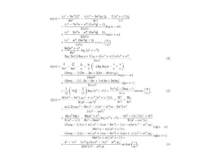
Second-order results: • We have obtained the solution explicitly, but it is too much complicated to exhibit here. • From the regularity of the geometry, “relaxation time” is uniquely determined. consistent with Heller-Janik, Baier et. al. , and Bhattacharyya et. al. 2 nd-order transport coefficient •

All-order results We can show the regularity by induction. n-th order Einstein’s equation: Diff eq. for bn = source which contains only k(<n)-th order metric “Regular enough” to show the regularity of bn and its arbitrary-order derivatives (except at the origin).

All-order results n-th order Einstein’s equation: Diff eq. for an = source which contains only k(<n)-th order metric and bn “Regular enough” to show the regularity of an and its arbitrary-order derivatives (except at the origin).

All-order results n-th order Einstein’s equation: Diff eq. for cn = source which contains only k(<n)-th order metric and an , bn Not always regular enough! n-th order transport coefficients comes here linearly Unique choice of the transport coefficients.

All-order results • There is no un-removable logarithmic singularity found on the FG coordinates. • We can make the geometry regular at all orders by choosing appropriate values of the transport coefficients. Our model is totally consistent and healthy!

Area of the apparent horizon greater! • This is consistent with the time evolution of the entropy density to the first order. • There is some discrepancy at the second order. However, it does not mean inconsistency immediately. From Hydro.

What we have done: • We constructed a consistent gravity dual of the Bjorken flow for the first time. (cf. Heller-Loganayagam-Spalinski-Surowka-Vazquez, ar. Xiv: 0805. 3774) • Our model is a concrete well-defined example of time-dependent Ad. S/CFT based on a well-controled approximation.

Time evolution of the stress tensor Hydrodynamics • hydrodynamic equation (energy-momentum conservation) • equation of state 　 (conformal invariance) • transport coefficients Our model 5 d Einstein’s eq. at the vicinity of the boundary Reguarity around the horizon Related to local thermal equilibrium

Discussion • The definition of the late-time approximation is a bit artificial. (τ-2/3 expansion with rτ1/3 = u fixed. ) • Is this a unique choice? • Can we derive it purely from gravity? • What is the physical meaning? • Is this related to the choice of the vacuum?

Discussion • At this stage, the connection among our method and other methods are not clear. • Kubo formula: • Quasi normal modes In this case, we impose the “ingoing boundary condition” at the horizon. regularity?

Comparison with Veronicka’s work Veronica’s work Our work const. + higher derivative (static) The leading order is already time-dependent Derivative expansion w. r. t 4 d coordinates by fixing r. Derivative expansion w. r. t 4 d coordinates by fixing u= rτ1/3. Full Minkowski spacetime Rindler wedge Expansion around a regular exact solution The leading-order metric is not an exact solution