A Guide To OptimizationBased MultiPeriod Planning December 2020

A Guide To Optimization-Based Multi-Period Planning December 2020 An updated version of a presentation at INFORMS Phoenix by Linus Schrage Monday, 5 November 2018 Keywords: Multi-period planning, Long range planning

Principal question: How to design and use optimization based multi-period planning models. Questions: info@lindo. com

Outline: History of Multi-Period Planning + Optimization. Backlogging, Lost Sales, the Basic Inventory Equation. Objectives: NPV and more. Multiple Dimensions of Modeling, Parkinson’s Law of Modeling. Rolling/Sliding Schedules and Combatting Nervousness. Inventory Types: Attrition, Perishable, Growing, FIFO vs. LIFO, Compressible. Planning Horizon Length, How to Choose. Period Length, Choosing. Start and End Conditions. Steady State and Steady Growth Rate Models, and Insight Provided. Resource, Precedence, & Changeover Constraints: How Not to Represent. Presenting Results of Multi-period Plans, Space-time Diagrams. Taxes, how to represent. Uncertainty: How to represent compactly.

History of Multi-Period Planning & Optimization Dates at least to biblical times. (According to G. Dantzig) The parable of Joseph interpreting the Pharaoh's dream about the seven fat cows and the seven lean cows. Joseph: Seven good years will be followed by seven years that are lean. Planning advice: Do multi-period planning. Build up inventories of grain during fat years. Pharaoh: That worked out great! Joseph, how did you know what approach to use? Joseph: . . Use lean year programming

History of Multi-Period Planning & Optimization, More Recently: Holt, Modigliani, Muth, & Simon Planning Model (as Quadratic Program) Done for a Pittsburgh Paint Company, 1955 Given demand forecasts for the next 12 months, for a single (aggregated) product, we have a single work force, What are our options for satisfying the (predictably) fluctuating demand? Decisions: Change work force level from period to period? Use overtime in some periods? Carry inventory, or back log demand? Hanssmann & Hess 1960: gave a more practical reformulation as an LP.

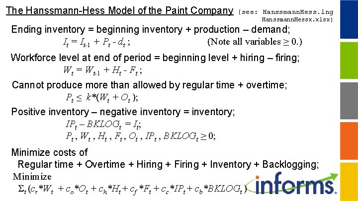
The Hanssmann-Hess Model of the Paint Company (see: Hanssmann. Hess. lng Hanssmann. Hessx. xlsx) Ending inventory = beginning inventory + production – demand; It = It-1 + Pt - dt ; (Note all variables ≥ 0. ) Workforce level at end of period = beginning level + hiring – firing; Wt = Wt-1 + Ht - Ft ; Cannot produce more than allowed by regular time + overtime; Pt ≤ k*(Wt + Ot ); Positive inventory – negative inventory = inventory; IPt – BKLOGt = It; Pt , Wt , Ht , Ft , Ot , IPt , BKLOGt ≥ 0; Minimize costs of Regular time + Overtime + Hiring + Firing + Inventory + Backlogging; Minimize Σt (cr*Wt + co*Ot + ch*Ht + cf *Ft + cc*IPt + cb*BKLOGt )

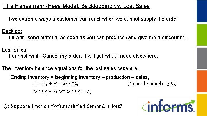
The Hanssmann-Hess Model, Backlogging vs. Lost Sales Two extreme ways a customer can react when we cannot supply the order: Backlog: I’ll wait, send material as soon as you can produce (and give me a discount? ). Lost Sales: I cannot wait. Cancel my order. I will get what I need elsewhere. The inventory balance equations for the lost sales case are: Ending inventory = beginning inventory + production – sales, It = It-1 + Pt – SALESt ; (Note all variables ≥ 0. ) SALESt + LOSTSALESt = dt; Q: Suppose fraction f of unsatisfied demand is lost?

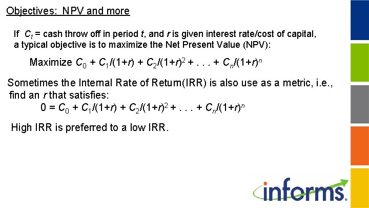
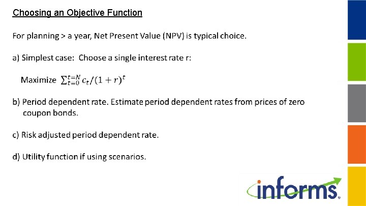
Objectives: NPV and more If Ct = cash throw off in period t, and r is given interest rate/cost of capital, a typical objective is to maximize the Net Present Value (NPV): Maximize C 0 + C 1/(1+r) + C 2/(1+r)2 +. . . + Cn/(1+r)n Sometimes the Internal Rate of Return(IRR) is also use as a metric, i. e. , find an r that satisfies: 0 = C 0 + C 1/(1+r) + C 2/(1+r)2 +. . . + Cn/(1+r)n High IRR is preferred to a low IRR.

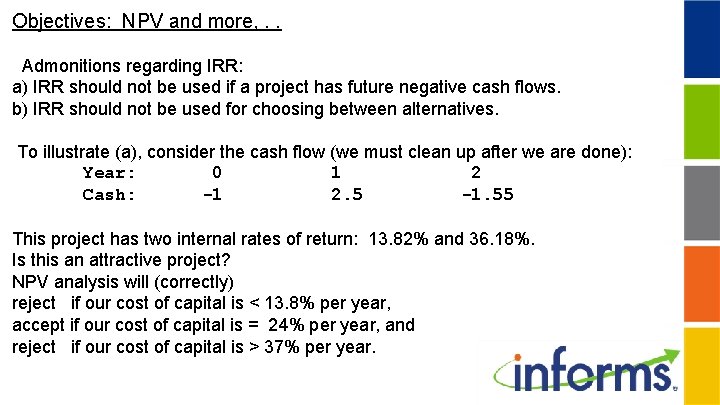
Objectives: NPV and more, . . Admonitions regarding IRR: a) IRR should not be used if a project has future negative cash flows. b) IRR should not be used for choosing between alternatives. To illustrate (a), consider the cash flow (we must clean up after we are done): Year: 0 1 2 Cash: -1 2. 5 -1. 55 This project has two internal rates of return: 13. 82% and 36. 18%. Is this an attractive project? NPV analysis will (correctly) reject if our cost of capital is < 13. 8% per year, accept if our cost of capital is = 24% per year, and reject if our cost of capital is > 37% per year.

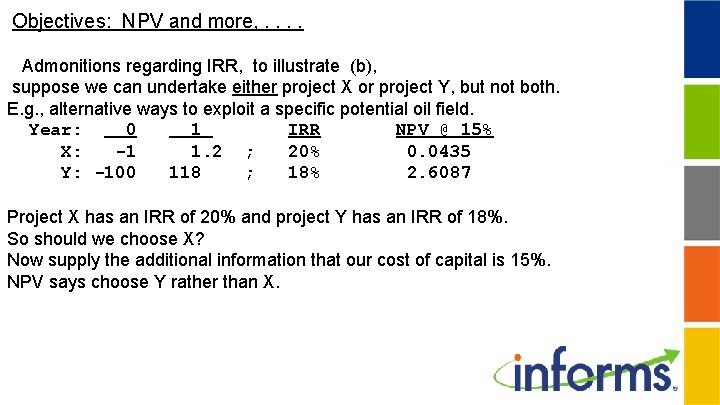
Objectives: NPV and more, . . Admonitions regarding IRR, to illustrate (b), suppose we can undertake either project X or project Y, but not both. E. g. , alternative ways to exploit a specific potential oil field. Year: 0 1 IRR NPV @ 15% X: -1 1. 2 ; 20% 0. 0435 Y: -100 118 ; 18% 2. 6087 Project X has an IRR of 20% and project Y has an IRR of 18%. So should we choose X? Now supply the additional information that our cost of capital is 15%. NPV says choose Y rather than X.

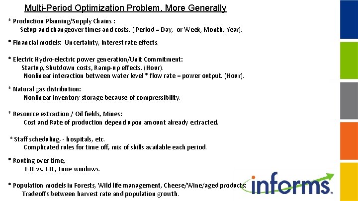
Multi-Period Optimization Problem, More Generally * Production Planning/Supply Chains : Setup and changeover times and costs. ( Period = Day, or Week, Month, Year). * Financial models: Uncertainty, interest rate effects. * Electric Hydro-electric power generation/Unit Commitment: Startup, Shutdown costs, Ramp-up effects. (Hour). Nonlinear interaction between water level * flow rate = power output. (Hour). * Natural gas distribution: Nonlinear inventory storage because of compressibility. * Resource extraction / Oil fields, Mines: Cost and Rate of production depend upon amount already extracted. * Staff scheduling, - hospitals, etc. Complicated rules for time off, mix of skills available each period. * Routing over time, FTL vs. LTL, Time windows. * Population models in Forests, Wild life management, Cheese/Wine/aged products: Tradeoffs between harvest rate and population growth.

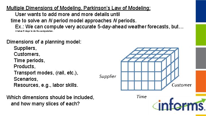
Multiple Dimensions of Modeling, Parkinson’s Law of Modeling: User wants to add more and more details until time to solve an N period model approaches N periods. Ex. : We can compute very accurate 5 -day-ahead weather forecasts, but… it takes 6 days to do the computation. Dimensions of a planning model: Suppliers, Customers, Time periods, Products, Transport modes, (rail, etc. ), Scenarios, Resources, e. g. , labor skills. Which dimensions should be included, and how many slices of each? Supplier Customer Time

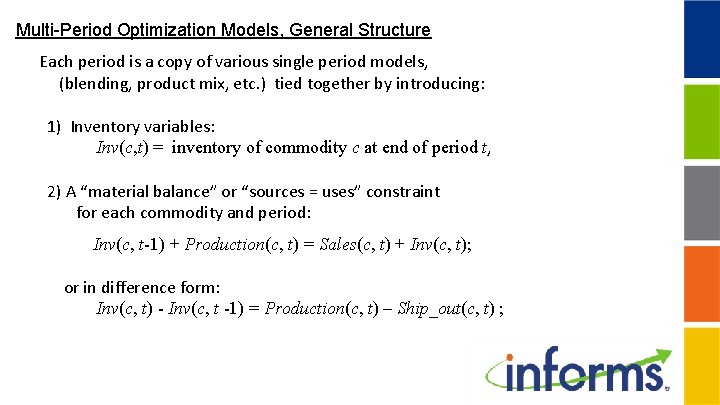
Multi-Period Optimization Models, General Structure Each period is a copy of various single period models, (blending, product mix, etc. ) tied together by introducing: 1) Inventory variables: Inv(c, t) = inventory of commodity c at end of period t, 2) A “material balance” or “sources = uses” constraint for each commodity and period: Inv(c, t-1) + Production(c, t) = Sales(c, t) + Inv(c, t); or in difference form: Inv(c, t) - Inv(c, t -1) = Production(c, t) – Ship_out(c, t) ;

Multi-Period Optimization Models, Complications & Issues * Rolling/Sliding Schedules and Nervousness. *Types of inventories: attrition, growth, FIFO vs. LIFO, perishable, compressible. *Planning horizon length * End effects, Choosing planning horizon, * Steady state and steady growth rate models, and the insight they provide. * Resource, precedence, & changeover constraints: a simple bad way, a better way. * How to present results of multi-period plans, space-time diagrams. * Taxes, how to represent. * Uncertainty: How to represent compactly.

Multi-Period Optimization Models, Common Features/Problem Rolling/Sliding Schedules Results from model are used in rolling/sliding fashion: Loop: 1) Solve an N period model, 2) Implement the results from the first one or two periods of solution; 3) Update forecasts, Slide the model forward one period, Repeat Problem: Model nervousness: As forecasts change, the recommended solution may change a lot. The folks “on the production floor” may be unhappy with the significant change in plans, period to period. Suppliers like to know your long run production plans. They will be unhappy if your plans change dramatically with each plan release.

Nervousness and Rolling/Sliding Schedules How to combat solution nervousness when using rolling or sliding schedules. Observation: For typical real planning problems, there are many (close to) optima. Approach used successfully in scheduling ships, plant closings/openings, production of breakfast cereal, by Brown, Dell, and Wood (1997), is to Specify a “reference” solution (e. g. , the solution from the run of previous month). Define secondary objective of minimize deviation of the current solution from reference. If zero weight on the secondary objective ==> theoretically optimal solution. If high weight on the secondary objective, ==> reference solution returned. If a modest weight on secondary objective, ==> alternate (almost) optimum close to reference solution.

Choosing a Planning Horizon Simple Suggestion: If solving an N+1 period problem and an N period problem give the same first period solution, then use N as the planning horizon. This may be too long or too short. Too long: Alternate optima, or close to alternate in which first period decisions are not the same. Too short: Adding November made no difference in the January solution, but when you added December, there was a big change in January solution. Note, there is a substantial literature on identifying planning horizons for moderately simple multi-period lotsizing problems using above rule.

Choosing a Planning Horizon General approach: N is a good planning horizon length if 1) Solve an N period problem; 2) Solve the two problems: A) For the decisions in the first period fixed, solve an N+K period problem, B) For the decisions in the first period not fixed, solve N+K period problem, If the costs of the solutions to A and B are not significantly different, then N is a reasonable planning horizon. Variation: If requiring integrality in first N+K periods, gives the same first period solution as requiring integrality in first N periods, then OK to require integrality in only first N periods.

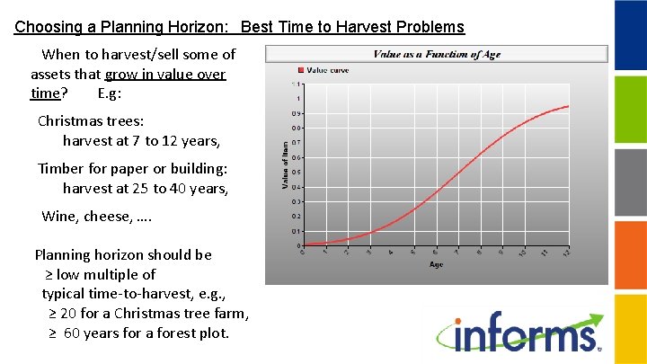
Choosing a Planning Horizon: Best Time to Harvest Problems When to harvest/sell some of assets that grow in value over time? E. g: Christmas trees: harvest at 7 to 12 years, Timber for paper or building: harvest at 25 to 40 years, Wine, cheese, …. Planning horizon should be ≥ low multiple of typical time-to-harvest, e. g. , ≥ 20 for a Christmas tree farm, ≥ 60 years for a forest plot.

Choosing a Period Length Examples: In scheduling daily work patterns at a telephone call center, distribution centers, etc. , breaks are a multiple of 15 minutes, so typical period length is 15 minutes. In scheduling nurses, a traditional period is a week. In scheduling electrical generators, it may take an hour to bring a generator up to full power, so a period might be an hour. Period length need not be constant, e. g. , Periods: 1 -4 = 1 quarter/3 months, Periods: 5 -6 = 1 year, Periods: 6 -7 = 2 years, Period 8 = 1 year repeated forever.

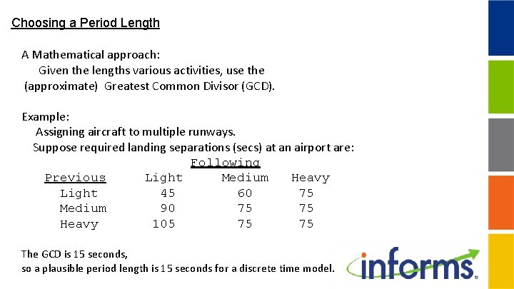
Choosing a Period Length A Mathematical approach: Given the lengths various activities, use the (approximate) Greatest Common Divisor (GCD). Example: Assigning aircraft to multiple runways. Suppose required landing separations (secs) at an airport are: Following Previous Light Medium Heavy Light 45 60 75 Medium 90 75 75 Heavy 105 75 75 The GCD is 15 seconds, so a plausible period length is 15 seconds for a discrete time model.

Multi-Period Optimization Models, Steady State Solutions Steady state solutions are sometimes of interest. Why? Easier to understand. Users like them, “There is a flight to Tucson every Tuesday. ” Easier to solve. May give “Insight”. Useful as the final period. Finding a Steady State Constant solution is conceptually simple: Make the ending conditions = beginning conditions, e. g. , the inventory levels. A slightly more general definition of steady state or stationarity is if the growth rate remains unchanged from one period to the next. Slightly more precisely, there is a scalar, λ, so that for every inventory or state c: INV( c, t) = λ * INV( c, t-1) ; Simple steady state has λ = 1;

Multi-Period Optimization Models, Steady State Solutions, Alternative Optima Suppose we require that the ending conditions = beginning conditions. This may result in alternate optima, which can increase solve time if solving an integer program. Example: We want find an optimal food menu for a 4 week period. There are various constraints such as nutritional requirements each day and variety constraints among days, e. g. , cannot serve the same meal two days in a row. If there are no day specific constraints, e. g. , must serve fish on Friday, then there will be 4*7 = 28 alternate optima. Another solution obtained from the previous by shifting the solution forward and around one day.

Steady State Solutions – Cyclic Solutions: Choosing a Cycle Length Simplest form of a steady state is to add a constraint that the end of the period state must equal the conditions at the beginning of the period. Sometimes is useful to allow the cycle length to be more than one period. This is particularly true in routing or staffing problems, e. g. , you might require that the solution repeat every four weeks rather than every week.

Population Models, Steady State Solutions A slightly more general definition of steady state or stationarity is if the growth rate remains unchanged from one period to the next. Consider a multi-period population model where: P(s, t) = population size of species s, in period t, where different species might be: 1 month-old cheese, 2 -month old rabbits, 3 -month old rabbits, 4 -month old foxes, 1 -year old pine trees, 2 -year old pine trees, etc.

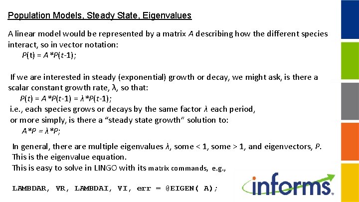
Population Models, Steady State, Eigenvalues A linear model would be represented by a matrix A describing how the different species interact, so in vector notation: P(t) = A*P(t-1); If we are interested in steady (exponential) growth or decay, we might ask, is there a scalar constant growth rate, λ, so that: P(t) = A*P(t-1) = λ*P(t-1); i. e. , each species grows or decays by the same factor λ each period, or more simply, is there a “steady state growth” solution to: A*P = λ*P; In general, there are multiple eigenvalues λ, some < 1, some > 1, and eigenvectors, P. This is the eigenvalue equation. This is easy to solve in LINGO with its matrix commands, e. g. , LAMBDAR, VR, LAMBDAI, VI, err = @EIGEN( A);

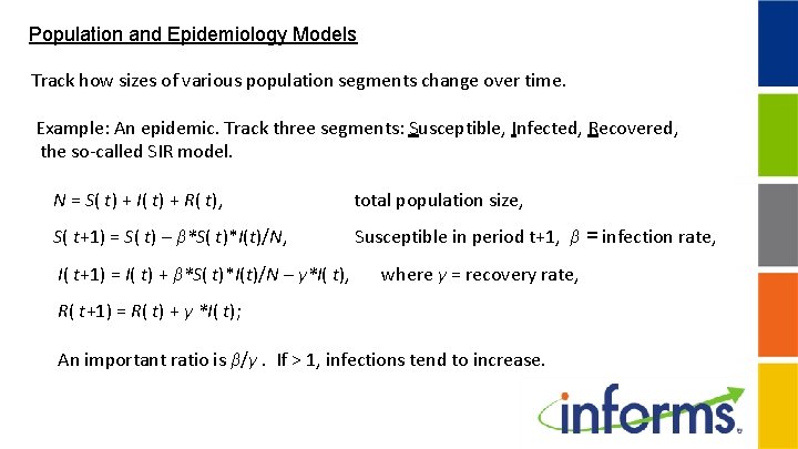
Population and Epidemiology Models Track how sizes of various population segments change over time. Example: An epidemic. Track three segments: Susceptible, Infected, Recovered, the so-called SIR model. N = S( t) + I( t) + R( t), total population size, S( t+1) = S( t) – β*S( t)*I(t)/N, Susceptible in period t+1, β = infection rate, I( t+1) = I( t) + β*S( t)*I(t)/N – γ*I( t), where γ = recovery rate, R( t+1) = R( t) + γ *I( t); An important ratio is β/γ. If > 1, infections tend to increase.

Multi-Period Planning, How to Choose Boundary Conditions? Ending conditions: If we arbitrarily terminate our planning model at year five in the future, then an optimal solution to our model may, in reality, be an optimal solution to how to go out of business in five years. Some of the options for handling the end effect are: a) Truncation (default). Simply drop from the model all periods beyond N. b) Primal limits. Place reasonable limits on inventories, etc. at the end of the final period. E. g. , in Pittsburgh Paint company, ending inventory was given a lower bound. c) Salvage values/ dual prices. Place reasonable salvage values on final inventories, etc. If you are an airline with fuel inventories, you may place a salvage value on fuel ending inventory.

Multi-Period Planning, How to Choose End Conditions? d) Infinite number of steady state periods. Final period of the model represents an infinite number of periods for which the same decision applies in every period to infinity. Net present value discounting is used in the objective function to make the final period comparable to the earlier finite periods. This approach used by: Carino et al. in their model of the Yasuda Kasai Insurance Company, Peiser and Andrus in their model of Texas real estate development, and Eppen, Martin, and Schrage in their model of General Motors production planning.

Multi-Period Planning, How to Choose Boundary Conditions? Beginning conditions: a) Use current state of real system. b) Start however you wish, but ending state must approximately match beginning state, e. g. , if trying to model steady state behavior. c) “Irregular Operations” (IROPS) is a standard term in airlines for a system for how to best recover after a disruption, typically bad weather. Problem: Given current state with resources (planes, crews, passengers) in the wrong place, what is the most efficient way of getting back on schedule? Priorities, decisions, costs: Get stranded passengers to their destinations, which flights to cancel, which planes and crews to fly from stranded location to where to get back on schedule by, say, Monday.

Modeling Taxes Essential tax computation equations are: Profitt Losst = Revenuet Expenset ; May need to enforce: Either Profitt or Losst = 0; Note, these are taxable revenues and expenses. Uses. Casht = Sources. Casht ; Uses. Casht = Tax. Ratet *Profitt + etc. Expenset = Depreciationt + etc. Complications: Depreciation, LIFO vs. FIFO, Loss carryforward, perhaps limited in number of years, -need to use idea of inventories that age.

Compressible Inventories, Limits on Inventory Change Rates Natural gas distributors may store gas in compressed form in large reservoirs in preparation for cold weather and related demand spikes. There are two interesting features because of the pressure in the reservoirs, there are limits on the rate at which inventory can be increased or decreased, and further, a) It gets harder to insert more gas when inventory is high. b) It gets harder to remove more gas when inventory is low. Key point: On a cold day when the demand is high, we may be in trouble, even if we have a sufficient supply of gas, but the pressure is not high enough to withdraw it a rapidly as needed. There are various approaches…

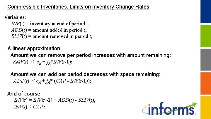
Compressible Inventories, Limits on Inventory Change Rates Variables: INV(t) = inventory at end of period t, ADD(t) = amount added in period t, RMV(t) = amount removed in period t, A linear approximation; Amount we can remove period increases with amount remaining: RMV(t) ≤ a. R + f. R*INV(t-1); Amount we can add period decreases with space remaining: ADD(t) ≤ a. A + f. A* (CAP - INV(t-1)); And of course: INV(t) = INV(t -1) + ADD(t) - RMV(t), INV(t) ≤ CAP ;

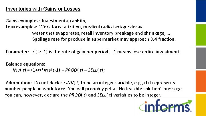
Inventories with Gains or Losses Gains examples: Investments, rabbits, … Loss examples: Work force attrition, medical radio-isotope decay, water that evaporates, retail inventory breakage and shrinkage, … Spoilage rate for produce in supermarket may approach 0. 4 fraction. Parameter: r ( ≥ -1) is the rate of gain period, -1 means lose entire investment. Balance equations: INV( t) = (1+r)*INV(t-1) + PROD( t) – SELL( t); Admonition: Do not declare INV( t) to be an integer variable, e. g. , if it represents number people in work force. You will probably get a “No feasible solution” message. You can, however, declare the PROD( t) and SELL( t) variables to be integer.

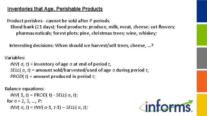
Inventories that Age, Perishable Products Product perishes - cannot be sold after P periods. Blood bank (21 days); food products: produce, milk, meat, cheese; cut flowers; pharmaceuticals; forest plots: pine, christmas trees; wine, whiskey; Interesting decisions: When should we harvest/sell trees, cheese, …? Variables: INV( a, t) = inventory of age a at end of period t, SELL( a, t) = amount sold/harvested/used of age a during period t, PROD( t) = amount produced in period t; Balance equations: INV( 1, t) = PROD( t) - SELL( a, t); for a = 2, 3, …, P: INV( a, t) = INV( a-1, t-1) – SELL( a, t);

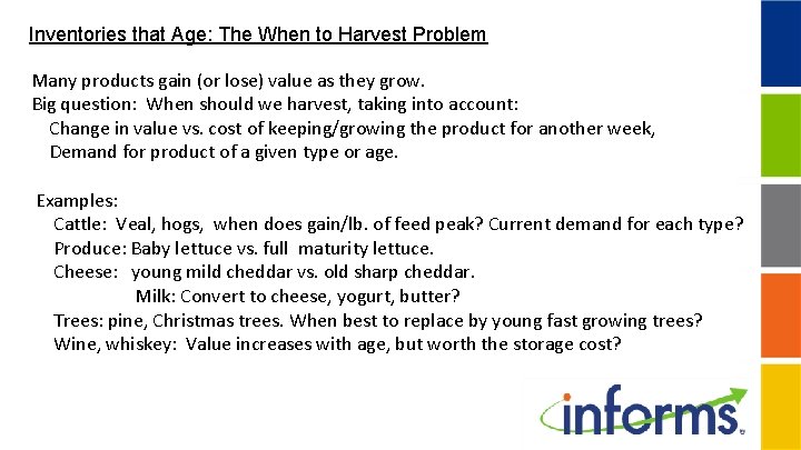
Inventories that Age: The When to Harvest Problem Many products gain (or lose) value as they grow. Big question: When should we harvest, taking into account: Change in value vs. cost of keeping/growing the product for another week, Demand for product of a given type or age. Examples: Cattle: Veal, hogs, when does gain/lb. of feed peak? Current demand for each type? Produce: Baby lettuce vs. full maturity lettuce. Cheese: young mild cheddar vs. old sharp cheddar. Milk: Convert to cheese, yogurt, butter? Trees: pine, Christmas trees. When best to replace by young fast growing trees? Wine, whiskey: Value increases with age, but worth the storage cost?

Precedence and Resource Constraints There are precedence constraints among activities in a number of situations: Air Traffic Congestion Modeling, A plane cannot enter sector j of flight until it finished sector j-1. Tank scheduling in process industries, A chemical batch cannot enter tank j of process until finishes j-1. Mining-open pit/cast, Block j cannot be removed until all blocks above removed. Petroleum extraction, Stage j of extraction with associated production rate cannot be entered until stage j-1 completed.

Multi-Period Optimization Models, Resource Extraction Notable feature: Cost/unit extracted and production rate from a location depends upon cumulative production from the location. Cost/unit may start high and then drop. In petroleum, cost/unit may start low, and then increase. Mining: Partition ore area into blocks, and define Parameters: PP = set of predecessors pairs. (i, j) in PP means j cannot be extracted before i is completed. Decision variables: z(j, t) = 1 if block j is extracted in period t, else 0; Crucial constraints: For all (i, j) in PP: Cannot extract block j unless i already extracted, z(j, t) ≤ ∑ s≤tz(j, s);

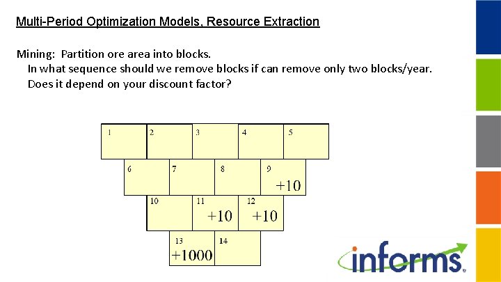
Multi-Period Optimization Models, Resource Extraction Mining: Partition ore area into blocks. In what sequence should we remove blocks if can remove only two blocks/year. Does it depend on your discount factor?

Precedence Constraints: How to Represent Usual notation: z( j, p) = 1 if task j is started in period p, else 0. Precedence: If i must be started no later than j, z( j, p) + z ( j, p-1) +. . . + z ( j, 1) ≤ z(i, p) + z (i, p-1) +. . . + z (i, 1), for p = 1, 2, . . . ; Better: Define the cumulative “done” variable: w(i, p) = 1 if task i is started in period p or earlier, else 0. = z(i, p) + z(i, p-1) +. . . + z (i, 1), = z(i, p) + w(i, p-1), **** Precedence: If i must be started no later than j, w( j, p) ≤ w(i, p), for p = 1, 2, . . . ; **** Simpler algebraically, and, branching in MIP search tree tends to be better.

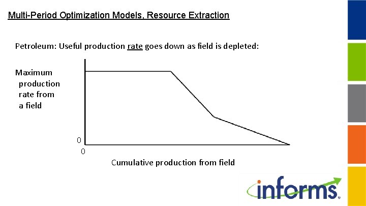
Multi-Period Optimization Models, Resource Extraction Petroleum: Useful production rate goes down as field is depleted: Maximum production rate from a field 0 0 Cumulative production from field

Multi-Period Optimization Models, Resource Extraction Petroleum: Partition extraction from a field into a number of stages (e. g. , 2 to 4). Define Parameters: PU(i, s) = maximum production period if field i is in stage s, PT(i, s) = total cumulative production in field i available in stage s, Decision variables: P(i, t, s) = actual production in field i in period t in stage s, z(i, t, s) = 1 if field i, in period t, enters stage s; presume a field can enter at most one stage period. Constraints: If we start stage s in period t, then previous stage must be exhausted: ∑r≤ t. P(i, r, s -1) ≥ PT(i, s -1)*z(i, t, s); Cannot produce more from a stage than available up to period t: ∑r≤ t. P(i, r, s) ≤ PT(i, s)* ∑r≤ t z(i, r, s); Cannot produce more than is available period: P(i, t, s) ≤ PU(i, s)*∑r≤ t z(i, r, s);

Resource Constraints, Continuous vs. Discrete Time For each job and machine combination, there is a processing time of the job on the specific machine, as well as a value of this assignment, So: Assign jobs to machines, and find a Sequence of jobs on each machine so that At most one job is assigned to a specific machine at a specific instant, and Each job is done in its time window, and the Value of the assignments is maximized;

Resource Constraints, Continuous vs. Discrete Time Job to Machine Assignment and Sequencing Jobs (trucks, ships, airplanes, patients, hotel guests. . . ) arrive over time at a facility (terminal, harbor, hospital, hotel, . . . ). Facility has a number of “machines”: docks, gates, operating rooms…. Examples: airplanes to parallel runways (gates, de-icing stations) at an airport, trucks or ships to docks at a freight terminal, hotel guests to hotel rooms, surgical procedures to operating rooms, manufacturing jobs to machines in a factory. Each machine can handle at most one job at a time. A job cannot be started before its arrival time. Each job has a due date by which its processing should be finished.

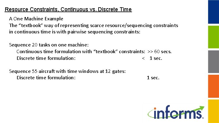
Resource Constraints, Continuous vs. Discrete Time A One Machine Example The “textbook” way of representing scarce resource/sequencing constraints in continuous time is with pairwise sequencing constraints: Sequence 20 tasks on one machine: Continuous time formulation with “textbook” constraints: >> 60 secs. Discrete time formulation: < 1 sec. Sequence 55 aircraft with time windows at 12 gates: Discrete time formulation: 1 sec.

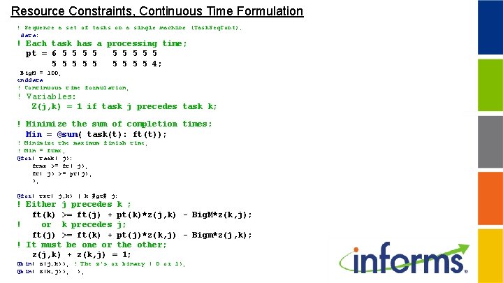
Resource Constraints, Continuous Time Formulation ! Sequence a set of tasks on a single machine (Task. Seq. Cont); data: ! Each task has a processing time; pt = 6 5 5 5 5 5 4; Big. M = 100; enddata ! Continuous time formulation; ! Variables: Z(j, k) = 1 if task j precedes task k; ! Minimize the sum of completion times; Min = @sum( task(t): ft(t)); ! Minimize the maximum finish time; ! Min = ftmx; @for( task( j): ftmx >= ft( j); ft( j) >= pt(j); ); @for( txt( j, k) | k #gt# j: ! Either j precedes k ; ft(k) >= ft(j) + pt(k)*z(j, k) - Big. M*z(k, j); ! or k precedes j; ft(j) >= ft(k) + pt(j)*z(k, j) - Bigm*z(j, k); ! It must be one or the other; z(j, k) + z(k, j) = 1; @bin( z(j, k)); ! The z's or binary ( 0 or 1); @bin( z(k, j)); );

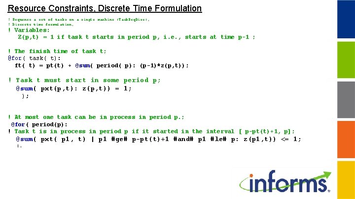
Resource Constraints, Discrete Time Formulation ! Sequence a set of tasks on a single machine (Task. Seq. Disc); ! Discrete time formulation; ! Variables: Z(p, t) = 1 if task t starts in period p, i. e. , starts at time p-1 ; ! The finish time of task t; @for( task( t): ft( t) = pt(t) + @sum( period( p): (p-1)*z(p, t)); ! Task t must start in some period p; @sum( pxt(p, t): z(p, t)) = 1; ); ! At most one task can be in process in period p. ; @for( period(p): ! Task t is in process in period p if it started in the interval [ p-pt(t)+1, p]; @sum( pxt( p 1, t) | p 1 #ge# p-pt(t)+1 #and# p 1 #le# p: z(p 1, t)) <= 1; );

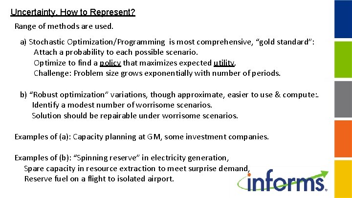
Uncertainty, How to Represent? Range of methods are used. a) Stochastic Optimization/Programming is most comprehensive, “gold standard”: Attach a probability to each possible scenario. Optimize to find a policy that maximizes expected utility. Challenge: Problem size grows exponentially with number of periods. b) “Robust optimization” variations, though approximate, easier to use & compute: . Identify a modest number of worrisome scenarios. Solution should be repairable under worrisome scenarios. Examples of (a): Capacity planning at GM, some investment companies. Examples of (b): “Spinning reserve” in electricity generation, Spare capacity in resource extraction to meet surprise demand, Reserve fuel on a flight to isolated airport.

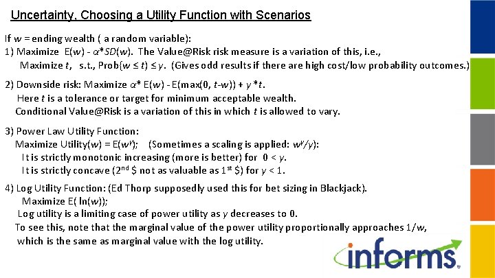
Uncertainty, Choosing a Utility Function with Scenarios If w = ending wealth ( a random variable): 1) Maximize E(w) - α*SD(w). The Value@Risk risk measure is a variation of this, i. e. , Maximize t, s. t. , Prob{w ≤ t) ≤ γ. (Gives odd results if there are high cost/low probability outcomes. ) 2) Downside risk: Maximize α* E(w) - E(max(0, t-w)) + γ *t. Here t is a tolerance or target for minimum acceptable wealth. Conditional Value@Risk is a variation of this in which t is allowed to vary. 3) Power Law Utility Function: Maximize Utility(w) = E(wγ); (Sometimes a scaling is applied: wγ/γ): It is strictly monotonic increasing (more is better) for 0 < γ. It is strictly concave (2 nd $ not as valuable as 1 st $) for γ < 1. 4) Log Utility Function: (Ed Thorp supposedly used this for bet sizing in Blackjack). Maximize E( ln(w)); Log utility is a limiting case of power utility as γ decreases to 0. To see this, note that the marginal value of the power utility proportionally approaches 1/w, which is the same as marginal value with the log utility.

Choosing an Objective Function

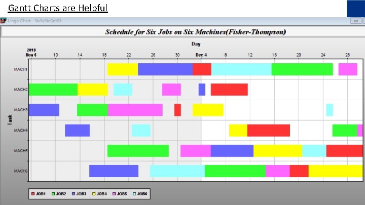
Displaying Time Based Results: Space-Time Diagrams * Gantt Charts * Time Conversion/Calendar Routines * *available in LINGO

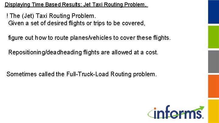
Displaying Time Based Results: Jet Taxi Routing Problem, ! The (Jet) Taxi Routing Problem. Given a set of desired flights or trips to be covered, figure out how to route planes/vehicles to cover these flights. Repositioning/deadheading flights are allowed at a cost. Sometimes called the Full-Truck-Load Routing problem.

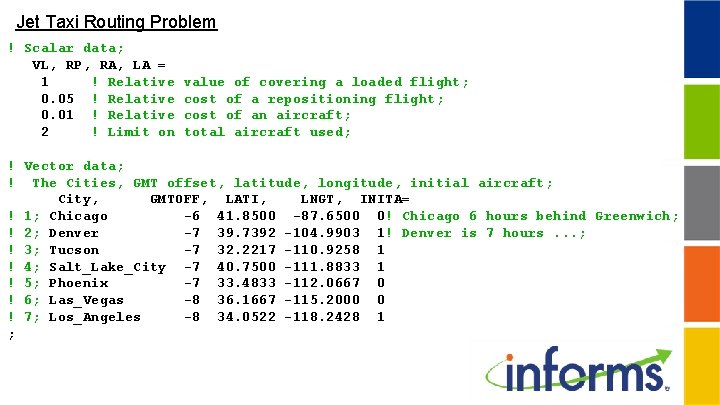
Jet Taxi Routing Problem ! Scalar data; VL, RP, RA, LA = 1 ! Relative 0. 05 ! Relative 0. 01 ! Relative 2 ! Limit on value of covering a loaded flight; cost of a repositioning flight; cost of an aircraft; total aircraft used; ! Vector data; ! The Cities, GMT offset, latitude, longitude, initial aircraft; City, GMTOFF, LATI, LNGT, INITA= ! 1; Chicago -6 41. 8500 -87. 6500 0! Chicago 6 hours behind Greenwich; ! 2; Denver -7 39. 7392 -104. 9903 1! Denver is 7 hours. . . ; ! 3; Tucson -7 32. 2217 -110. 9258 1 ! 4; Salt_Lake_City -7 40. 7500 -111. 8833 1 ! 5; Phoenix -7 33. 4833 -112. 0667 0 ! 6; Las_Vegas -8 36. 1667 -115. 2000 0 ! 7; Los_Angeles -8 34. 0522 -118. 2428 1 ;

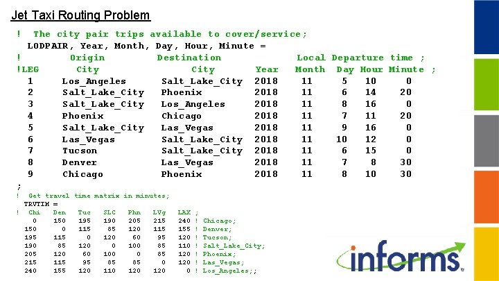
Jet Taxi Routing Problem ! The city pair trips available to cover/service; LODPAIR, Year, Month, Day, Hour, Minute = ! Origin Destination Local Departure time ; !LEG City Year Month Day Hour Minute ; 1 Los_Angeles Salt_Lake_City 2018 11 5 10 0 2 Salt_Lake_City Phoenix 2018 11 6 14 20 3 Salt_Lake_City Los_Angeles 2018 11 8 16 0 4 Phoenix Chicago 2018 11 7 11 20 5 Salt_Lake_City Las_Vegas 2018 11 9 16 0 6 Las_Vegas Salt_Lake_City 2018 11 10 12 0 7 Tucson Salt_Lake_City 2018 11 6 15 0 8 Denver Las_Vegas 2018 11 7 8 30 9 Chicago Phoenix 2018 11 8 10 30 ; ! Get travel time matrix in minutes; TRVTIM = ! Chi Den Tuc SLC Phn LVg 0 150 195 190 205 215 150 0 115 85 120 115 195 115 0 120 60 95 190 85 120 0 100 85 205 120 60 100 0 85 215 115 95 85 85 0 240 155 120 110 120 LAX 240 155 120 110 120 0 ; ! ! ! ! Chicago; Denver; Tucson; Salt_Lake_City; Phoenix; Las_Vegas; Los_Angeles; ;

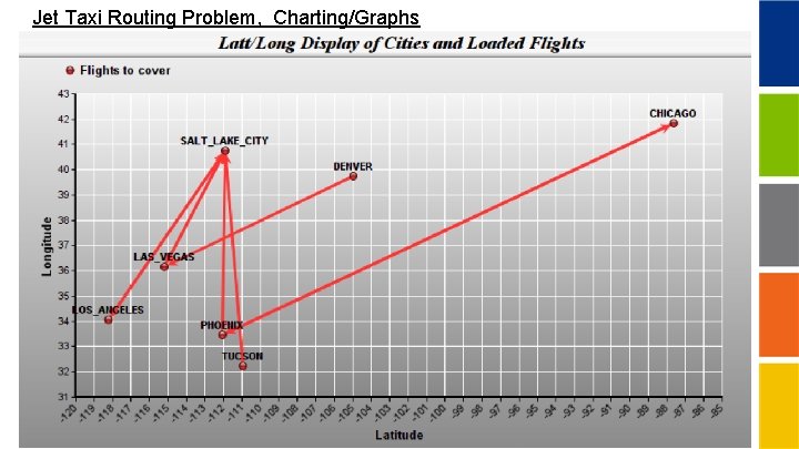
Jet Taxi Routing Problem, Charting/Graphs

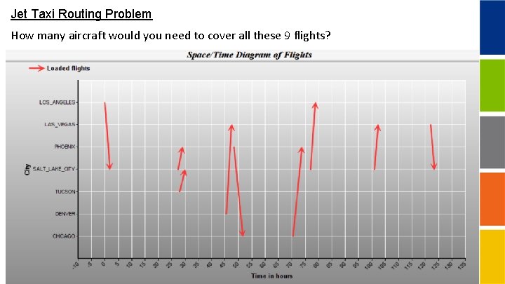
Jet Taxi Routing Problem How many aircraft would you need to cover all these 9 flights?

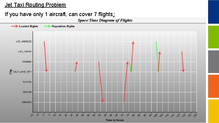
Jet Taxi Routing Problem If you have only 1 aircraft, can cover 7 flights:

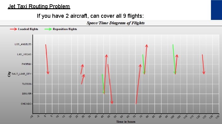
Jet Taxi Routing Problem If you have 2 aircraft, can cover all 9 flights:

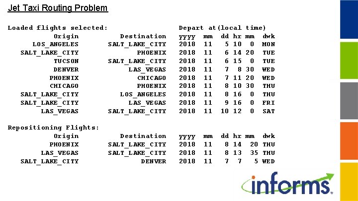
Jet Taxi Routing Problem Loaded flights selected: Origin Destination LOS_ANGELES SALT_LAKE_CITY PHOENIX TUCSON SALT_LAKE_CITY DENVER LAS_VEGAS PHOENIX CHICAGO PHOENIX SALT_LAKE_CITY LOS_ANGELES SALT_LAKE_CITY LAS_VEGAS SALT_LAKE_CITY Depart at(local yyyy mm dd hr 2018 11 5 10 2018 11 6 14 2018 11 6 15 2018 11 7 8 2018 11 7 11 2018 11 8 10 2018 11 8 16 2018 11 9 16 2018 11 10 12 Repositioning Flights: Origin PHOENIX LAS_VEGAS SALT_LAKE_CITY yyyy 2018 Destination SALT_LAKE_CITY DENVER mm 11 11 11 time) mm dwk 0 MON 20 TUE 30 WED 20 WED 30 THU 0 FRI 0 SAT dd hr mm 8 14 20 8 13 35 7 7 5 dwk THU WED

Gantt Charts are Helpful

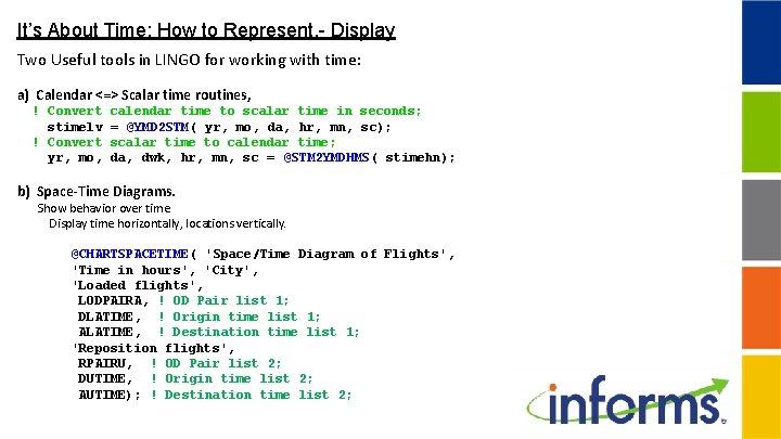
It’s About Time: How to Represent, - Display Two Useful tools in LINGO for working with time: a) Calendar <=> Scalar time routines, ! Convert stimelv ! Convert yr, mo, calendar time to scalar time in seconds; = @YMD 2 STM( yr, mo, da, hr, mn, sc); scalar time to calendar time; da, dwk, hr, mn, sc = @STM 2 YMDHMS( stimehn); b) Space-Time Diagrams. Show behavior over time. Display time horizontally, locations vertically. @CHARTSPACETIME( 'Space/Time Diagram of Flights', 'Time in hours', 'City', 'Loaded flights', LODPAIRA, ! OD Pair list 1; DLATIME, ! Origin time list 1; ALATIME, ! Destination time list 1; 'Reposition flights', RPAIRU, ! OD Pair list 2; DUTIME, ! Origin time list 2; AUTIME); ! Destination time list 2;

Thank you for your attention! Comments or Questions, linus@lindo. com linus. schrage@chicagobooth. edu

Some References - 1 Dimitris Bertsimas, Guglielmo Lulli, Amedeo Odoni, (2011) An Integer Optimization Approach to Large-Scale Air Traffic Flow Management. Operations Research 59(1): 211 -227. Brown, G. G. , R. F. Dell, and R. K. Wood (1997), “Optimization and Persistence”, Interfaces, vol. 27, No. 5, (Sept‑Oct), pp. 15‑ 37. Cariño, D. Myers, and W. Ziemba (1998), "Concepts, Technical Issues, and Uses of the Russell-Yasuda Kasai Financial Planning Model", Operations Research, vol. 46, no. 4 (Jul. -Aug), pp. 450 -462. Chand, S. , Morton, T. E. , Proth, J. M. , Existence of forecast horizons in undiscounted discrete-time lot size models, Operations Research 38 (1990) 884 -892. Ding, X. and M. Puterman(2002), “The Censored Newsvendor and the Optimal Acquisition of Information”, Operations Research, vol. 50, no. 3, pp. 517 -527. Eppen, G. , R. Martin, and L. Schrage(1989), “A Scenario Approach to Capacity Planning”, Operations Research, vol. 37, no. 4, 517 -527. Fisher, M. and A. Raman(1996), “Reducing the Cost of Demand Uncertainty Through Accurate Response to Early Sales”, Operations Research, vol. 44 , no. 1, pp. 8799. Grinold, R. and K. Marshall (1977 ), Manpower Planning Models, North-Holland. Hanssmann, F. and S. Hess, “A Linear Programming Approach to Production and Employment Scheduling”, Management Technology, vol. 1, No. 1 (Jan. , 1960), pp. 46 -51. Holt, C. C. , Modigliani, F. , and H. A. Simon, (1955), “A linear decision rule for production and employment scheduling”, Management Science , October, vol. 2, no. 1, pp. 159 -177. Holt, C. C. , Modigliani, F. , and Muth, J. , (1955), “Derivation of a linear decision rule for production and employment”, Management Science , October, vol. 2, no. 2, pp. 1 -30. Knowles, T. , and J. Wirick, (1998), "The Peoples Gas Light and Coke Company Plans Gas Supply", Interfaces, vol. 28, no. 5 (Sep-Oct), pp. 1 -12. Nahmias, S. , 2011, Perishable Inventory Systems, Springer. Peiser, R. , and S. Andrus, (1983) “Phasing of Income-Producing Real Estate”, Interfaces, vol. 13, no. 5 (Oct), pp. 1 -9.

Some References-2 Schrage, L. (2018), Optimization Modeling with LINGO, (chap. 9), LINDO Systems. Zipkin, P. (2000), Foundations of Inventory Management, Mc. Graw-Hill.