A GlobalLocal Optimization Framework for Simultaneous MultiMode MultiCorner

A Global-Local Optimization Framework for Simultaneous Multi-Mode Multi-Corner Clock Skew Variation Reduction Kwangsoo Han, Andrew B. Kahng, Jongpil Lee, Jiajia Li and Siddhartha Nath VLSI CAD LABORATORY, UC San Diego / VLSI CAD Laboratory -1 -

Outline n Motivation n Related Work n Our Optimization Framework n Experimental Setup and Results n Conclusions -2 -
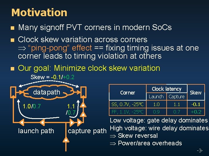
Motivation n Many signoff PVT corners in modern So. Cs n Clock skew variation across corners “ping-pong” effect == fixing timing issues at one corner leads to timing violation at others Our goal: Minimize clock skew variation n Skew = -0. 1/+0. 2 datapath 1. 0 /0. 7 launch path Corner 1. 1 /0. 7 Clock latency Skew Launch Capture SS, 0. 7 V, -25°C 1. 0 1. 1 -0. 1 FF, 1. 1 V, -25°C 0. 9 0. 7 +0. 2 Low voltage: gate delay dominates capture path High voltage: wire delay dominates Skew reversal Power/area overheads -3 -

Outline n Motivation n Related Work n Our Optimization Framework n Experimental Setup and Results n Conclusions -4 -
![Related Work Skew minimization at multiple corners n n [Cho 05] perform temperature-aware skew Related Work Skew minimization at multiple corners n n [Cho 05] perform temperature-aware skew](http://slidetodoc.com/presentation_image_h2/68b7e9f00b474ce3648cf14b058d0c70/image-5.jpg)
Related Work Skew minimization at multiple corners n n [Cho 05] perform temperature-aware skew reduction based on an improved DME [Lung 10] minimize the worst clock skew across corners with delay correlation factors Skew variation minimization across corners n n n [Restle 01] propose two-level non-tree structure, in which mesh is applied at bottom level [Su 01] use mesh for top-level of clock network [Rajaram 04] insert crosslinks in a clock tree to minimize skew variation Our work: systematic optimization framework for minimization of clock skew variation in clock tree -5 -

Skew Variation Reduction Problem r n At C’ : C’’ Skewi, j. C’ C’ max C At C : C’ Skew C i, j … i ∑ j r: root; i, j: sinks -6 -

Outline n Motivation n Related Work n Our Optimization Framework n Experimental Setup and Results n Conclusions -7 -
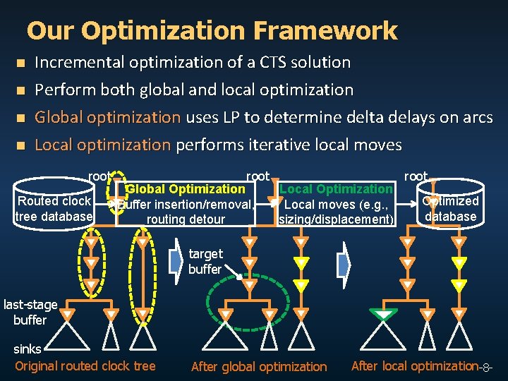
Our Optimization Framework n n Incremental optimization of a CTS solution Perform both global and local optimization Global optimization uses LP to determine delta delays on arcs Local optimization performs iterative local moves root Routed clock tree database root Global Optimization Buffer insertion/removal, routing detour Local Optimization Local moves (e. g. , sizing/displacement) root Optimized database target buffer last-stage buffer sinks Original routed clock tree After global optimization After local optimization-8 -

Global Optimization: LP n n Formulate linear program to minimize skew variation Determine the delta delay on each arc at each corner Based on LUTs to insert/remove buffer and detour wires Discreteness of buffer delays ECO feasibility is important Ø (1) Minimize number of ECO changes Ø (2) Sweep U for solution with minimum skew variation Ø (3) Ensure no skew degradation Ø (4) Maximum clock latency constraint Ø (1, 5, 6) Improve ECO feasibility -9 -
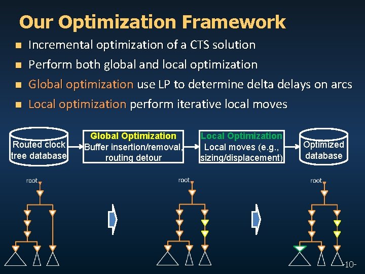
Our Optimization Framework n n Incremental optimization of a CTS solution Perform both global and local optimization Global optimization use LP to determine delta delays on arcs Local optimization perform iterative local moves Routed clock tree database Global Optimization Buffer insertion/removal, routing detour Local Optimization Local moves (e. g. , sizing/displacement) Optimized database -10 -
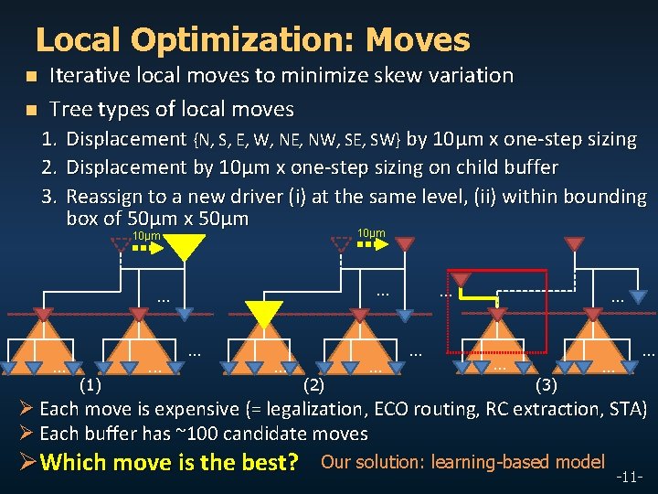
Local Optimization: Moves n n Iterative local moves to minimize skew variation Tree types of local moves 1. Displacement {N, S, E, W, NE, NW, SE, SW} by 10μm x one-step sizing 2. Displacement by 10μm x one-step sizing on child buffer 3. Reassign to a new driver (i) at the same level, (ii) within bounding box of 50μm x 50μm 10μm . . (1) . . (2) . . . . (3) . . . Ø Each move is expensive (= legalization, ECO routing, RC extraction, STA) Ø Each buffer has ~100 candidate moves ØWhich move is the best? Our solution: learning-based model -11 -
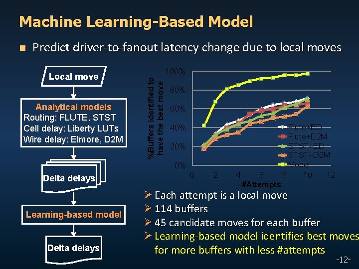
Machine Learning-Based Model Predict driver-to-fanout latency change due to local moves Local move Analytical models Routing: FLUTE, STST Cell delay: Liberty LUTs Wire delay: Elmore, D 2 M 100% %Buffers identified to have the best move n 80% 60% 40% 20% 0% Delta delays Learning-based model Delta delays 0 2 4 6 #Attempts Flute+ED Flute+D 2 M STST+ED STST+D 2 M Model 8 10 12 Ø Each attempt is a local move Ø 114 buffers Ø 45 candidate moves for each buffer Ø Learning-based model identifies best moves for more buffers with less #attempts -12 -

Outline n Motivation n Related Work n Our Optimization Framework n Experimental Setup and Results n Conclusions -13 -
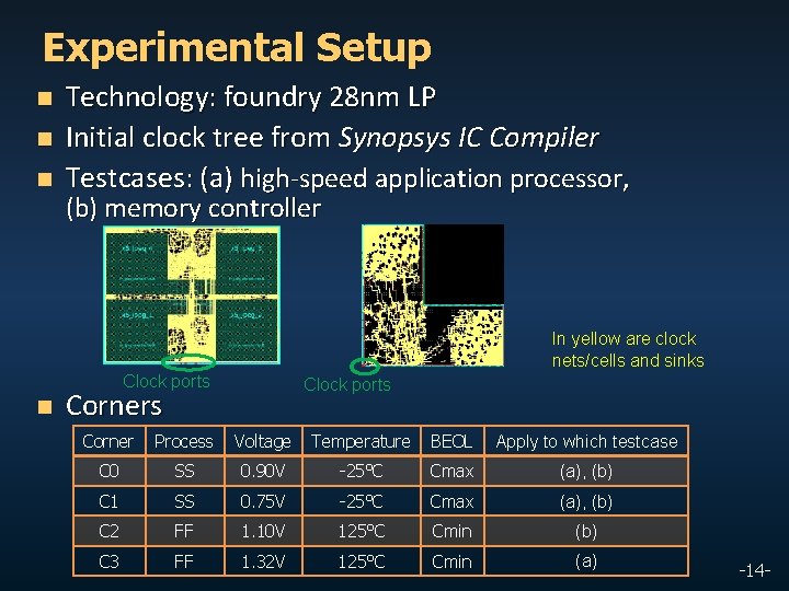
Experimental Setup n n n Technology: foundry 28 nm LP Initial clock tree from Synopsys IC Compiler Testcases: (a) high-speed application processor, (b) memory controller In yellow are clock nets/cells and sinks Clock ports n Clock ports Corner Process Voltage Temperature BEOL Apply to which testcase C 0 SS 0. 90 V -25°C Cmax (a), (b) C 1 SS 0. 75 V -25°C Cmax (a), (b) C 2 FF 1. 10 V 125°C Cmin (b) C 3 FF 1. 32 V 125°C Cmin (a) -14 -
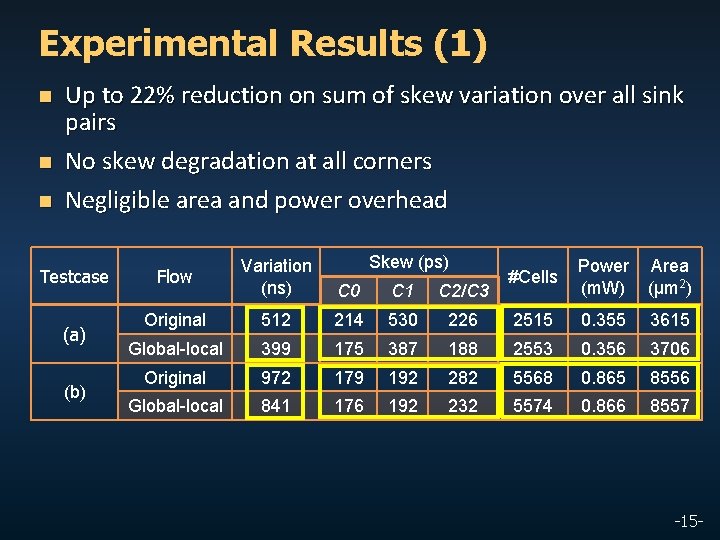
Experimental Results (1) n Up to 22% reduction on sum of skew variation over all sink pairs No skew degradation at all corners n Negligible area and power overhead n Testcase (a) (b) Skew (ps) Flow Variation (ns) #Cells Power (m. W) Area (μm 2) C 0 C 1 C 2/C 3 Original 512 214 530 226 2515 0. 355 3615 Global-local 399 175 387 188 2553 0. 356 3706 Original 972 179 192 282 5568 0. 865 8556 Global-local 841 176 192 232 5574 0. 866 8557 -15 -
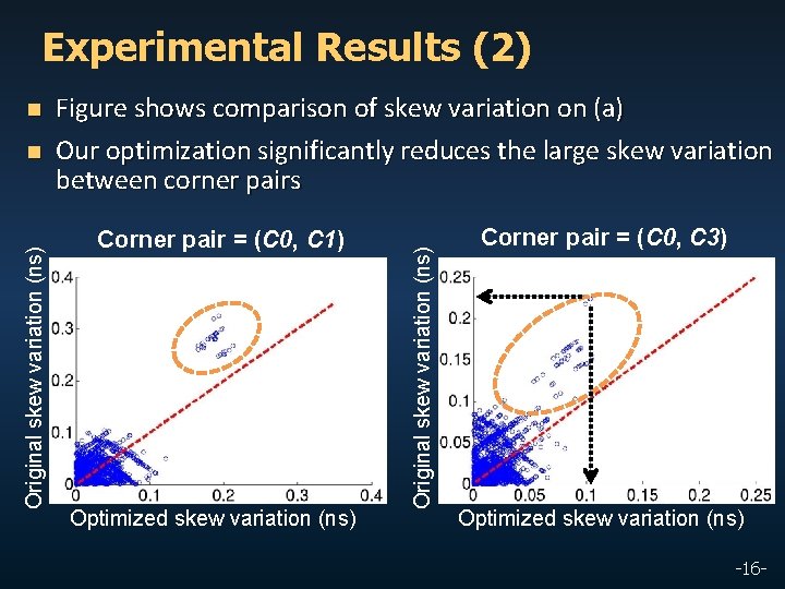
Experimental Results (2) Original skew variation (ns) n Figure shows comparison of skew variation on (a) Our optimization significantly reduces the large skew variation between corner pairs Corner pair = (C 0, C 1) Optimized skew variation (ns) Original skew variation (ns) n Corner pair = (C 0, C 3) Optimized skew variation (ns) -16 -

Outline n Motivation n Related Work n Our Optimization Framework n Experimental Setup and Results n Conclusions -17 -
Conclusion and Future Works n n n First framework to minimize sum of skew variation over all sink pairs in a clock tree Up to 22% reduction of the sum of skew variation Future works – Study resultant power and area benefits – Model to predict a buffer location for minimum skew over a continuous range of possible locations Thank You! -18 -

Backup Slides -19 -
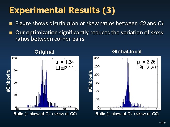
Experimental Results (3) n n Figure shows distribution of skew ratios between C 0 and C 1 Our optimization significantly reduces the variation of skew ratios between corner pairs Global-local μ = 1. 34 2 = 3. 21 �� Ratio (= skew at C 1 / skew at C 0) #Sink pairs Original μ = 2. 26 2 = 2. 26 �� Ratio (= skew at C 1 / skew at C 0) -20 -
- Slides: 20