A Gentle Introduction to Linear Mixed Modeling and

A Gentle Introduction to Linear Mixed Modeling and PROC MIXED Richard Charnigo Associate Professor of Statistics and Biostatistics Director of Statistics and Psychometrics Core, CDART RJCharn 2@aol. com

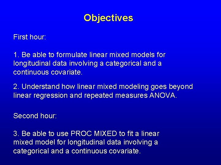
Objectives First hour: 1. Be able to formulate linear mixed models for longitudinal data involving a categorical and a continuous covariate. 2. Understand how linear mixed modeling goes beyond linear regression and repeated measures ANOVA. Second hour: 3. Be able to use PROC MIXED to fit a linear mixed model for longitudinal data involving a categorical and a continuous covariate.

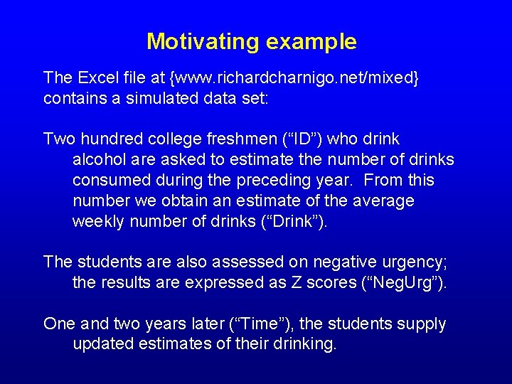
Motivating example The Excel file at {www. richardcharnigo. net/mixed} contains a simulated data set: Two hundred college freshmen (“ID”) who drink alcohol are asked to estimate the number of drinks consumed during the preceding year. From this number we obtain an estimate of the average weekly number of drinks (“Drink”). The students are also assessed on negative urgency; the results are expressed as Z scores (“Neg. Urg”). One and two years later (“Time”), the students supply updated estimates of their drinking.

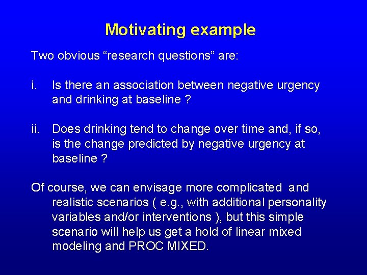
Motivating example Two obvious “research questions” are: i. Is there an association between negative urgency and drinking at baseline ? ii. Does drinking tend to change over time and, if so, is the change predicted by negative urgency at baseline ? Of course, we can envisage more complicated and realistic scenarios ( e. g. , with additional personality variables and/or interventions ), but this simple scenario will help us get a hold of linear mixed modeling and PROC MIXED.

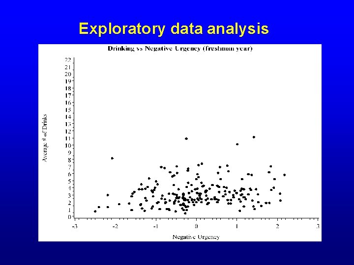
Exploratory data analysis Before pursuing linear mixed (or other statistical) modeling, we are well-advised to engage in exploratory data analysis. This can alert us to any gross mistakes in the data set, heretofore undetected, which may compromise our work. This can also suggest a structure for the linear mixed model and help us to anticipate what the results should be.

Exploratory data analysis

Exploratory data analysis

Exploratory data analysis

Exploratory data analysis

Exploratory data analysis The scatterplots suggest the following: • There are some outlying values, and drinking is not normally distributed, but there are not any values that are obviously fabricated or miskeyed. • There appears to be a positive association between drinking and negative urgency at baseline, which strengthens over time as those higher in negative urgency seem to be drinking more in later years. The latter impression is also conveyed by the plot of means and standard errors.

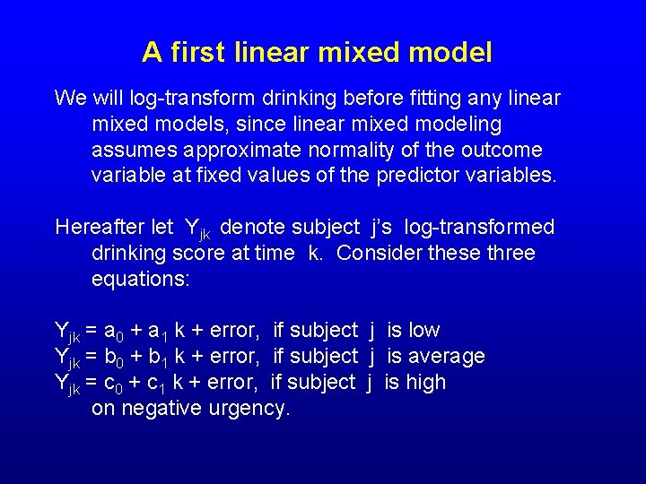
A first linear mixed model We will log-transform drinking before fitting any linear mixed models, since linear mixed modeling assumes approximate normality of the outcome variable at fixed values of the predictor variables. Hereafter let Yjk denote subject j’s log-transformed drinking score at time k. Consider these three equations: Yjk = a 0 + a 1 k + error, if subject j is low Yjk = b 0 + b 1 k + error, if subject j is average Yjk = c 0 + c 1 k + error, if subject j is high on negative urgency.

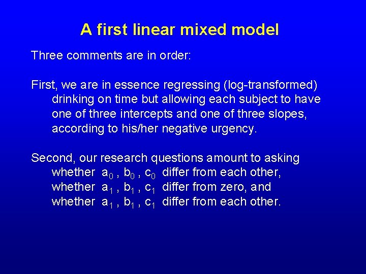
A first linear mixed model Three comments are in order: First, we are in essence regressing (log-transformed) drinking on time but allowing each subject to have one of three intercepts and one of three slopes, according to his/her negative urgency. Second, our research questions amount to asking whether a 0 , b 0 , c 0 differ from each other, whether a 1 , b 1 , c 1 differ from zero, and whether a 1 , b 1 , c 1 differ from each other.

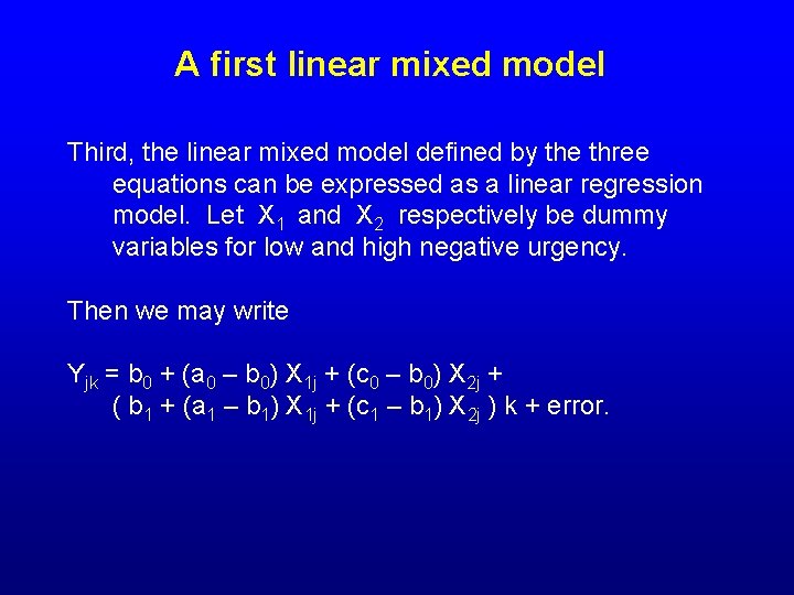
A first linear mixed model Third, the linear mixed model defined by the three equations can be expressed as a linear regression model. Let X 1 and X 2 respectively be dummy variables for low and high negative urgency. Then we may write Yjk = b 0 + (a 0 – b 0) X 1 j + (c 0 – b 0) X 2 j + ( b 1 + (a 1 – b 1) X 1 j + (c 1 – b 1) X 2 j ) k + error.

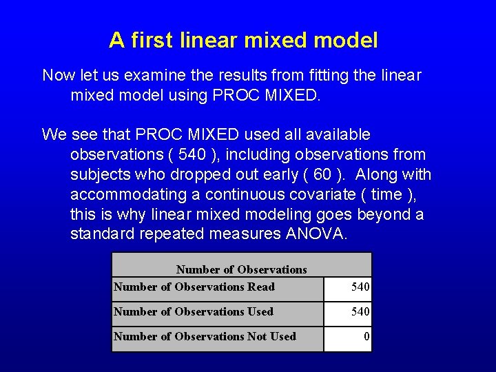
A first linear mixed model Now let us examine the results from fitting the linear mixed model using PROC MIXED. We see that PROC MIXED used all available observations ( 540 ), including observations from subjects who dropped out early ( 60 ). Along with accommodating a continuous covariate ( time ), this is why linear mixed modeling goes beyond a standard repeated measures ANOVA. Number of Observations Read 540 Number of Observations Used 540 Number of Observations Not Used 0

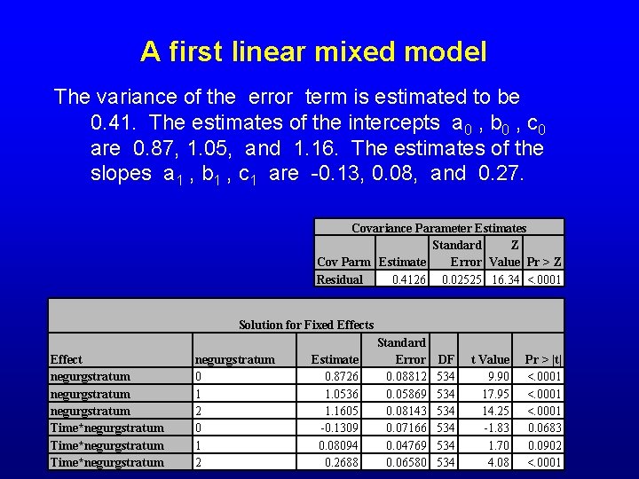
A first linear mixed model The variance of the error term is estimated to be 0. 41. The estimates of the intercepts a 0 , b 0 , c 0 are 0. 87, 1. 05, and 1. 16. The estimates of the slopes a 1 , b 1 , c 1 are -0. 13, 0. 08, and 0. 27. Covariance Parameter Estimates Standard Z Cov Parm Estimate Error Value Pr > Z Residual 0. 4126 0. 02525 16. 34 <. 0001 Solution for Fixed Effects Effect negurgstratum Time*negurgstratum 0 1 2 Estimate 0. 8726 1. 0536 1. 1605 -0. 1309 0. 08094 0. 2688 Standard Error 0. 08812 0. 05869 0. 08143 0. 07166 0. 04769 0. 06580 DF 534 534 534 t Value 9. 90 17. 95 14. 25 -1. 83 1. 70 4. 08 Pr > |t| <. 0001 0. 0683 0. 0902 <. 0001

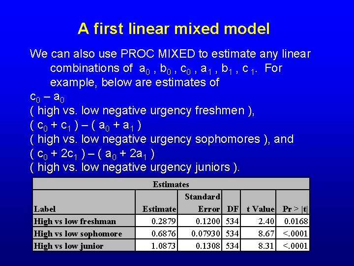
A first linear mixed model We can also use PROC MIXED to estimate any linear combinations of a 0 , b 0 , c 0 , a 1 , b 1 , c 1. For example, below are estimates of c 0 – a 0 ( high vs. low negative urgency freshmen ), ( c 0 + c 1 ) – ( a 0 + a 1 ) ( high vs. low negative urgency sophomores ), and ( c 0 + 2 c 1 ) – ( a 0 + 2 a 1 ) ( high vs. low negative urgency juniors ). Label High vs low freshman High vs low sophomore High vs low junior Estimates Standard Estimate Error 0. 2879 0. 1200 0. 6876 0. 07930 1. 0873 0. 1308 DF t Value Pr > |t| 534 2. 40 0. 0168 534 8. 67 <. 0001 534 8. 31 <. 0001

A second linear mixed model As noted earlier, our first linear mixed model can be expressed as a linear regression model. How, then, does linear mixed modeling go beyond linear regression ? The answer is that we may also allow each subject to have his/her own personal intercept and slope, not merely choose from among three intercepts and three slopes. The personal intercept and slope may be related to negative urgency and to unmeasured or unmeasurable characteristics.

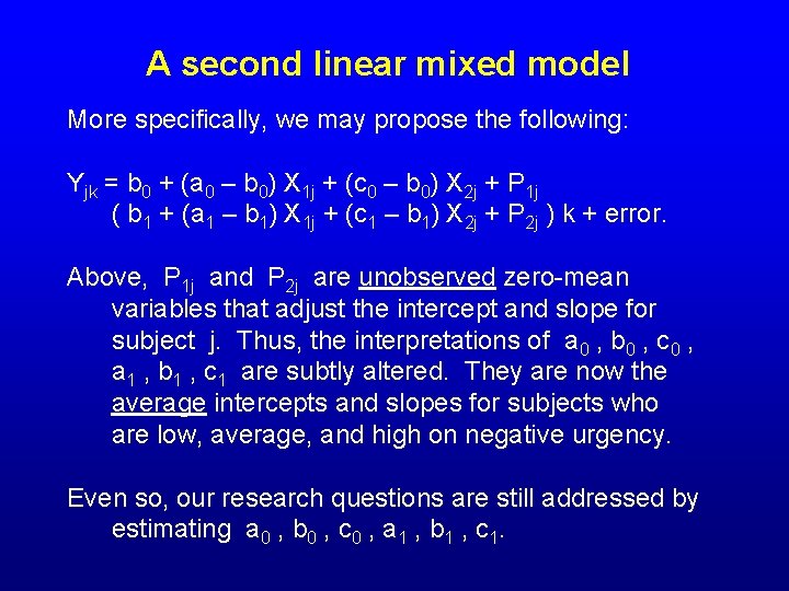
A second linear mixed model More specifically, we may propose the following: Yjk = b 0 + (a 0 – b 0) X 1 j + (c 0 – b 0) X 2 j + P 1 j ( b 1 + (a 1 – b 1) X 1 j + (c 1 – b 1) X 2 j + P 2 j ) k + error. Above, P 1 j and P 2 j are unobserved zero-mean variables that adjust the intercept and slope for subject j. Thus, the interpretations of a 0 , b 0 , c 0 , a 1 , b 1 , c 1 are subtly altered. They are now the average intercepts and slopes for subjects who are low, average, and high on negative urgency. Even so, our research questions are still addressed by estimating a 0 , b 0 , c 0 , a 1 , b 1 , c 1.

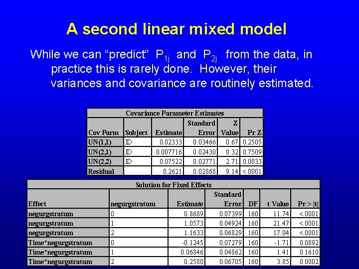
A second linear mixed model While we can “predict” P 1 j and P 2 j from the data, in practice this is rarely done. However, their variances and covariance are routinely estimated. Covariance Parameter Estimates Standard Z Cov Parm Subject Estimate Error Value UN(1, 1) ID 0. 02333 0. 03466 0. 67 UN(2, 1) ID 0. 007716 0. 02430 0. 32 UN(2, 2) ID 0. 07522 0. 02771 2. 71 Residual 0. 2621 0. 02868 9. 14 Pr Z 0. 2505 0. 7509 0. 0033 <. 0001 Solution for Fixed Effects Effect negurgstratum Time*negurgstratum 0 1 2 Estimate 0. 8689 1. 0573 1. 1633 -0. 1245 0. 06846 0. 2580 Standard Error 0. 07399 0. 04924 0. 06829 0. 07279 0. 04862 0. 06705 DF 160 160 160 t Value 11. 74 21. 47 17. 04 -1. 71 1. 41 3. 85 Pr > |t| <. 0001 0. 0892 0. 1610 0. 0002

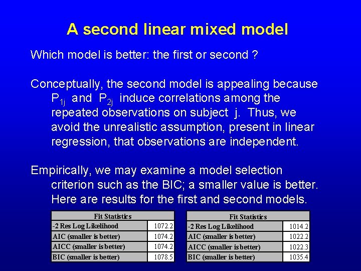
A second linear mixed model Which model is better: the first or second ? Conceptually, the second model is appealing because P 1 j and P 2 j induce correlations among the repeated observations on subject j. Thus, we avoid the unrealistic assumption, present in linear regression, that observations are independent. Empirically, we may examine a model selection criterion such as the BIC; a smaller value is better. Here are results for the first and second models. Fit Statistics -2 Res Log Likelihood AIC (smaller is better) AICC (smaller is better) BIC (smaller is better) 1072. 2 1074. 2 1078. 5 Fit Statistics -2 Res Log Likelihood AIC (smaller is better) AICC (smaller is better) BIC (smaller is better) 1014. 2 1022. 3 1035. 4

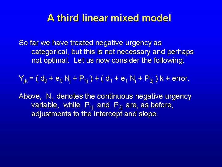
A third linear mixed model So far we have treated negative urgency as categorical, but this is not necessary and perhaps not optimal. Let us now consider the following: Yjk = ( d 0 + e 0 Nj + P 1 j ) + ( d 1 + e 1 Nj + P 2 j ) k + error. Above, Nj denotes the continuous negative urgency variable, while P 1 j and P 2 j are, as before, adjustments to the intercept and slope.

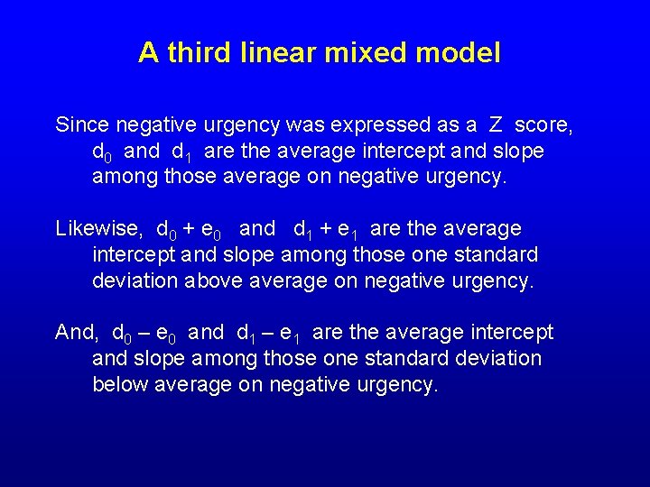
A third linear mixed model Since negative urgency was expressed as a Z score, d 0 and d 1 are the average intercept and slope among those average on negative urgency. Likewise, d 0 + e 0 and d 1 + e 1 are the average intercept and slope among those one standard deviation above average on negative urgency. And, d 0 – e 0 and d 1 – e 1 are the average intercept and slope among those one standard deviation below average on negative urgency.

A third linear mixed model We estimate the variances and covariance of P 1 j and P 2 j as well as estimating d 0 , e 0 , d 1 , e 1. Covariance Parameter Estimates Standard Z Error Value Pr Z 0. 03453 0. 57 0. 2859 Cov Parm UN(1, 1) Subject ID Estimate 0. 01952 UN(2, 1) ID 0. 005827 0. 02425 0. 24 0. 8101 UN(2, 2) ID 0. 07199 0. 02743 2. 62 0. 0043 0. 2633 0. 02885 9. 13 <. 0001 Residual Solution for Fixed Effects Effect Intercept Neg. Urg Time Neg. Urg*Time Estimate 1. 0414 Standard Error DF 0. 03495 198 t Value 29. 79 Pr > |t| <. 0001 0. 1152 0. 03613 160 3. 19 0. 0017 0. 07230 0. 03438 178 2. 10 0. 0369 0. 1446 0. 03533 160 4. 09 <. 0001

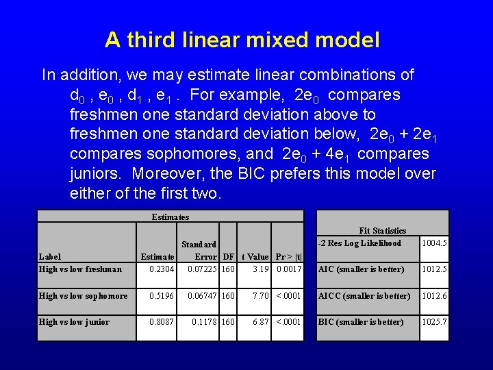
A third linear mixed model In addition, we may estimate linear combinations of d 0 , e 0 , d 1 , e 1. For example, 2 e 0 compares freshmen one standard deviation above to freshmen one standard deviation below, 2 e 0 + 2 e 1 compares sophomores, and 2 e 0 + 4 e 1 compares juniors. Moreover, the BIC prefers this model over either of the first two. Estimates Label High vs low freshman Standard Estimate Error DF t Value Pr > |t| 0. 2304 0. 07225 160 3. 19 0. 0017 Fit Statistics -2 Res Log Likelihood 1004. 5 AIC (smaller is better) 1012. 5 High vs low sophomore 0. 5196 0. 06747 160 7. 70 <. 0001 AICC (smaller is better) 1012. 6 High vs low junior 0. 8087 0. 1178 160 6. 87 <. 0001 BIC (smaller is better) 1025. 7

What’s next ? After a short break, we will launch SAS and examine the PROC MIXED implementations of the three linear mixed models as well as the exploratory data analyses that preceded them. In addition to replicating the results shown in this presentation, we will discuss some potentially useful modifications of and additions to the SAS code ( e. g. , how to estimate other linear combinations of coefficients in PROC MIXED).