A gentle introduction to Gaussian distribution Review Random
A gentle introduction to Gaussian distribution
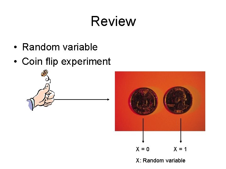
Review • Random variable • Coin flip experiment X=0 X=1 X: Random variable
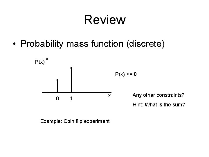
Review • Probability mass function (discrete) P(x) >= 0 0 1 x Any other constraints? Hint: What is the sum? Example: Coin flip experiment
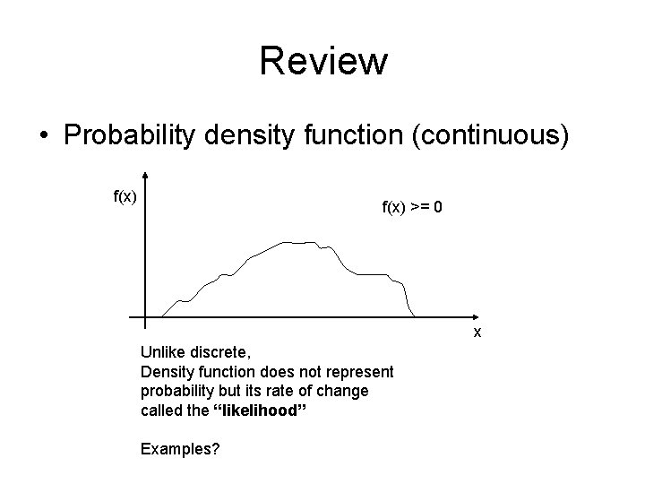
Review • Probability density function (continuous) f(x) >= 0 x Unlike discrete, Density function does not represent probability but its rate of change called the “likelihood” Examples?
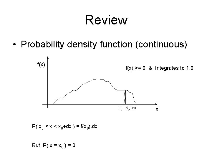
Review • Probability density function (continuous) f(x) >= 0 & Integrates to 1. 0 x 0 X 0+dx P( x 0 < x 0+dx ) = f(x 0). dx But, P( x = x 0 ) = 0 x
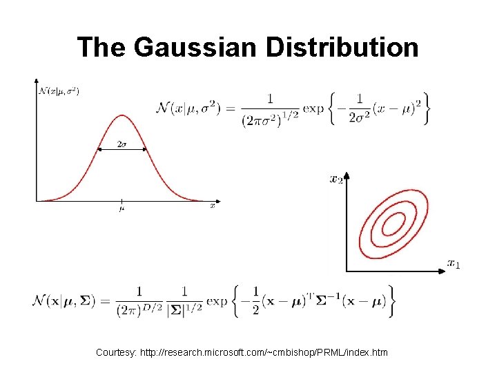
The Gaussian Distribution Courtesy: http: //research. microsoft. com/~cmbishop/PRML/index. htm
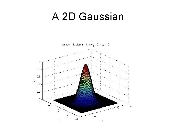
A 2 D Gaussian
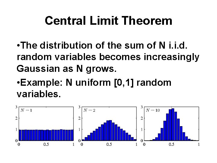
Central Limit Theorem • The distribution of the sum of N i. i. d. random variables becomes increasingly Gaussian as N grows. • Example: N uniform [0, 1] random variables.
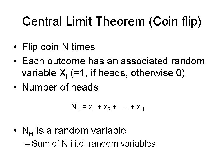
Central Limit Theorem (Coin flip) • Flip coin N times • Each outcome has an associated random variable Xi (=1, if heads, otherwise 0) • Number of heads NH = x 1 + x 2 + …. + x. N • NH is a random variable – Sum of N i. i. d. random variables
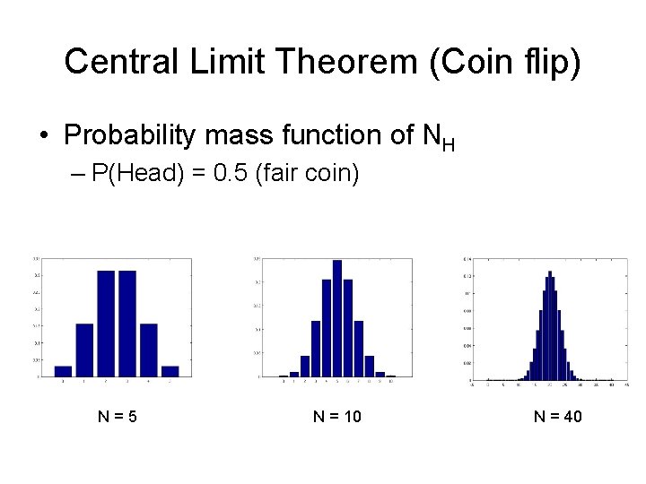
Central Limit Theorem (Coin flip) • Probability mass function of NH – P(Head) = 0. 5 (fair coin) N=5 N = 10 N = 40
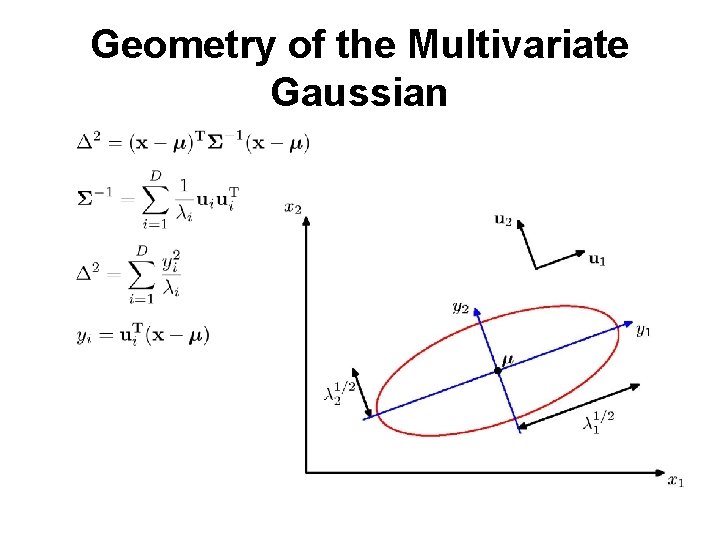
Geometry of the Multivariate Gaussian
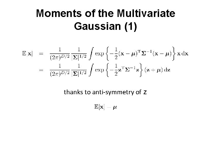
Moments of the Multivariate Gaussian (1) thanks to anti-symmetry of z
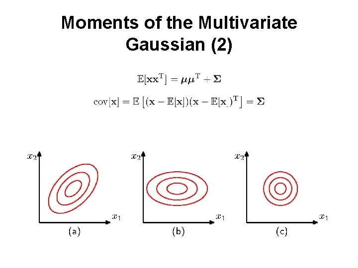
Moments of the Multivariate Gaussian (2)
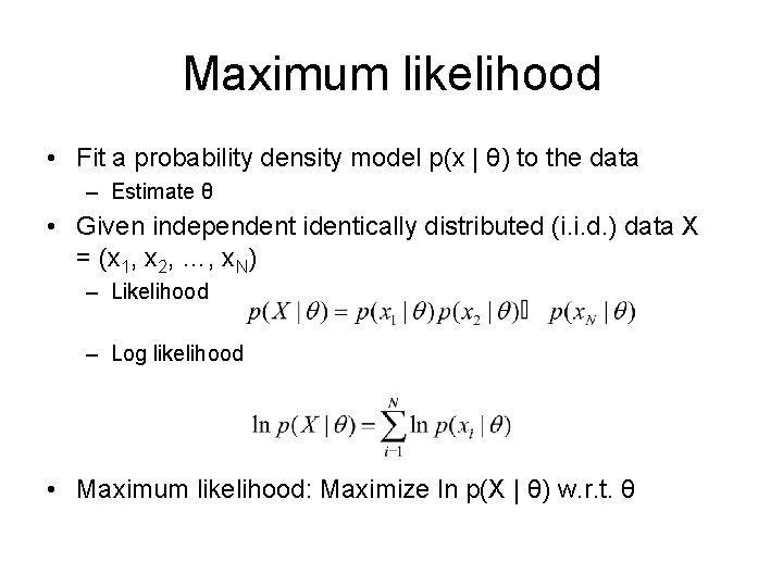
Maximum likelihood • Fit a probability density model p(x | θ) to the data – Estimate θ • Given independent identically distributed (i. i. d. ) data X = (x 1, x 2, …, x. N) – Likelihood – Log likelihood • Maximum likelihood: Maximize ln p(X | θ) w. r. t. θ
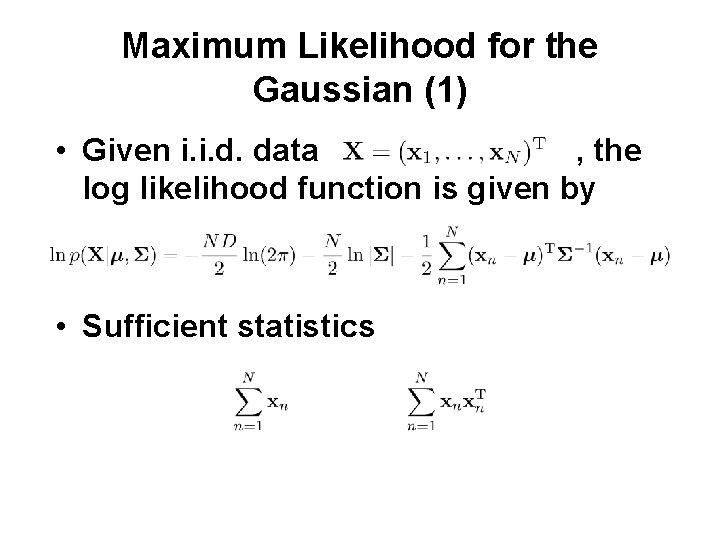
Maximum Likelihood for the Gaussian (1) • Given i. i. d. data , the log likelihood function is given by • Sufficient statistics
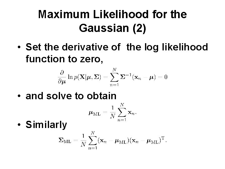
Maximum Likelihood for the Gaussian (2) • Set the derivative of the log likelihood function to zero, • and solve to obtain • Similarly
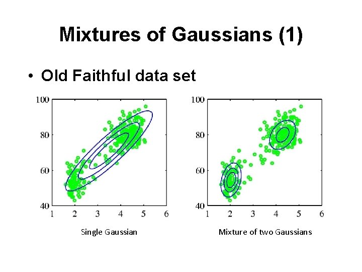
Mixtures of Gaussians (1) • Old Faithful data set Single Gaussian Mixture of two Gaussians
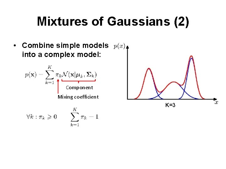
Mixtures of Gaussians (2) • Combine simple models into a complex model: Component Mixing coefficient K=3
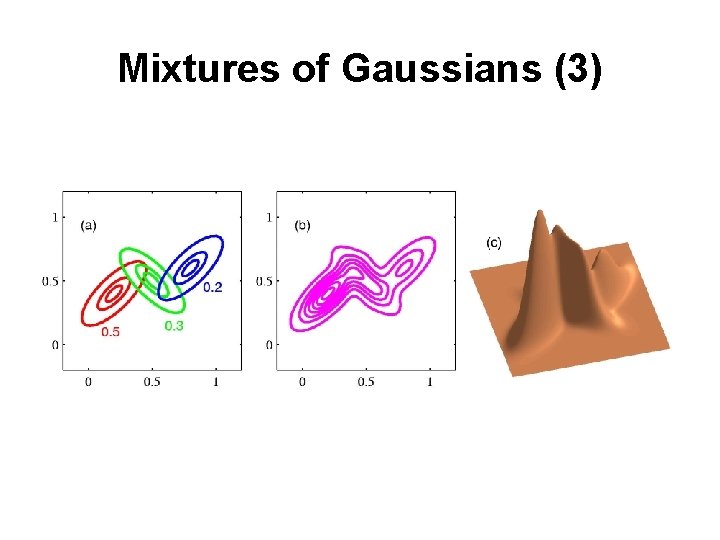
Mixtures of Gaussians (3)
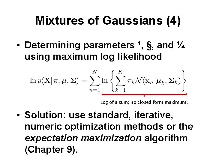
Mixtures of Gaussians (4) • Determining parameters ¹, §, and ¼ using maximum log likelihood Log of a sum; no closed form maximum. • Solution: use standard, iterative, numeric optimization methods or the expectation maximization algorithm (Chapter 9).

Thank you!
- Slides: 21