A FeatureSpaceBased Indicator Kriging Approach for Remote Sensing

A Feature-Space-Based Indicator Kriging Approach for Remote Sensing Image Classification Ke-Sheng Cheng Department of Bioenvironmental Systems Engineering National Taiwan University

Image Classification Statistical pattern recognition techniques are widely used for landuse/land cover classification. Some supervised classification algorithms Parametric Approach Maximum likelihood classifier Bayes classifier Non-parametric Approach Nearest Neighbour classifier Artificial Neural network classifier

ANN Classifiers ANN classifiers do not consider classification features as having probability distributions, and therefore, classification is not explicitly probability-based. In a loosely defined sense, ANN classification is a process of searching optimal solution of weight vector that minimizes the sum of squared errors between network and desired output responses.

ANN Classifiers It has been shown that the output of a backpropagation network can approximate the posterior density function, if its activation function is capable of representing the a posteriori probability function and the number of training samples is sufficiently large (Lee et al. , 1991). Manry et al. (1996) also showed that a neural network can approximate the minimum mean square estimator arbitrarily well, provided that it is of adequate size and is well-trained.

ANN Classifiers Egmont-Petersen et al. (2002) point out that ANNs suffer from what is known as the black-box problem: given any input a corresponding output is produced, but it cannot be elucidated why this decision was reached, how reliable it is, etc.

Image Classification The work of image classification can be considered as partitioning a hyperspace using discriminant rules established by samples. Each sample point in feature space is labeled a class index.

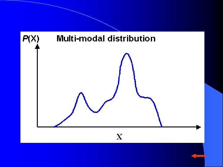
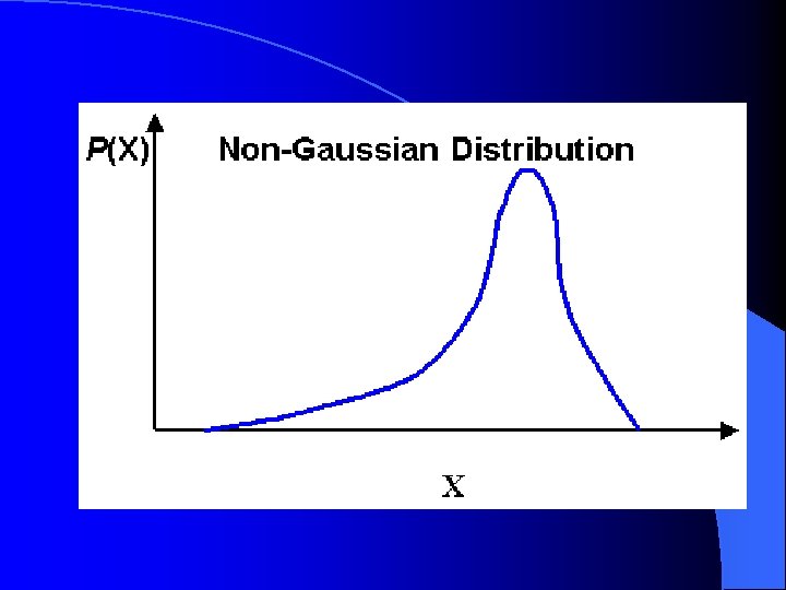
Difficulties Encountered In Application of Parametric Approaches Application of parametric approaches require knowledge of probability distribution of classification features. Classification features often have finite mixture distributions (multi-modal class densities). The class distribution may be non-Gaussian.

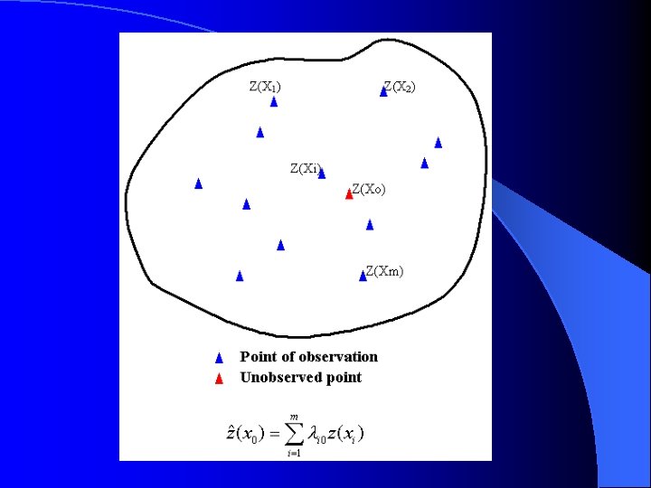
Geostatistical Approach of Spatial Estimation Geostatistics is a set of techniques, often referred to as kriging methods, which utilize the spatial covariance function or the semivariogram for spatial data analysis. Ordinary kriging yields best linear unbiased estimator (BLUE). Indicator kriging yields estimate of the probability distribution at specified locations.

Since probability density and correlation structure between classification features are insightful, probability-based classification methods are appealing to many researchers and practitioners. The work of probability-based classification can be conceived as a spatial estimation problem for which the estimates are probabilities that a pixel with certain feature -vector belongs to different classes.

Ordinary Kriging Ordinary kriging assumes second-order stationary properties for the random field {Z(x), x }

Properties of OK Estimates Unbiased i. e. Minimum variance of estimation error Conditional minimization Minimizing

Ordinary Kriging System Semi-variogram

Typical Form of A Variogram characterizes the spatial variation of a random field.

Matrix Form of OK System

Indicator Kriging Indicator kriging is a method of spatial estimation that yields an estimate of probability distribution function of the random variable of interest. Consider a random field of k classes where Ω represents the spatial domain of the random field. A total number of n features are used for classification of the k classes. For convenience of illustration, let’s assume k = 3 and n = 2. From a set of training pixels, we first establish the k-class scatter plot in feature space.

Scatter Plot in Feature Space

Indicator Variable For a continuous random field, the indicator variable can be used to estimate the distribution of the random variable by using a set of cutoff values. The indicator variable at location x is defined as where is a selected cutoff value.

The weighted average of indicator variables is an estimate of the cumulative probability, i. e. , If Z(xj), j = 1, 2, …, N, are mutually independent, then j = 1/N. For a random field with spatial autocorrelation characteristics, indicator variogram must be established and used to estimate the cumulative probability of the random variable at unobserved locations.

Indicator Variable for Categorical Random Field Similar to the case of continuous random field, the indicator variable can be used to estimate the probability that a pixel belongs to a certain class for categorical random field. Let the indicator variable be defined as wherere presents the j-th class and represents the pixel at location x. is the value of the indicator variable related to the j-th class.

The weighted average of values of indicator variables is an estimate of the probability that a pixel belongs to the j-th class, i. e.

Transforming Classification into Estimation The work of remote sensing image classification assigns one class identity to each pixel in the image. Class identities are categorical data and are non-continuous in geographical and feature spaces. Thus, spatial estimation of class identity in space is logically incorrect.

In order to transform the work of image classification into an estimation problem, two factors need to be considered. a non-categorical measure that associates with class identities. a space in which the chosen measure is continuous and spatial estimation of the chosen measure will be made.

In this study we adopt the classprobabilities, i. e. the probability that a pixel belongs to certain classes, as our spatial estimation parameters. Since spatial discontinuity of landcover often occurs in geographical space due to human activities, our estimation of class-probabilities takes place in a feature space rather than a geographical space.

Spatial discontinuity in geographical space (a) An image in geographical space with four types of landcover (shown in different patterns). Marked symbols represent training data points.

Spatial continuity in feature space (b) Distribution of training data in a two dimensional feature space.

Consider an image classification problem of k classes using m classification features. A random field represents the distribution of class identity in an m-dimensional spatial domain. For convenience of illustration, let’s assume k = 3 and m = 2. From a set of training pixels, we first establish the 3 -class scatter plot in feature space.

A three-class scatter plot in twodimensional feature space

In order to estimate the class probabilities in feature space, we then transform the threeclass scatter plot in two-dimensional feature space into three two-class scatter plots (binary scatter plots) corresponding to each of the three individual classes. For each binary scatter plot, we consider the spatial distribution of indicator variables as a random field associated with that particular class.

Class-specific Indicator Variable Scatter Plot in Feature Space Three-class scatter plot of indicator variables in two dimensional feature space. Class-specific Scatter plot of indicator variables (Binary Scatter Plots) Class-1 Class-2 Class-3

By conducting ordinary kriging for each class of indicator variables in feature space, we obtain the probability that the pixel of interest belongs to each individual class. Class assignment of the pixel of interest is done based on the following criterion If max , then assign to class.

Study Area and Image Data A study area of approximately 70 km 2 mostly within the Taipei city was selected for test of the proposed indicator kriging classification approach. Four major landcover types – water, woods, grass lands, and built-up areas – were identified due to the relatively simple landuse condition within the study area.

Multispectral SPOT satellite images acquired on December 24, 2001 was used for landcover classification. Sets of training and verification pixels were selected. In order to graphically illustrate the scattering of classified pixels in feature space by Gaussian-based maximum likelihood and indicator kriging classification methods we use only green (0. 50 0. 59 m) and infrared (0. 79 0. 89 m) spectral bands of SPOT images as classification features.

SPOT image of the study area (b) Green band (a) Infrared band

Non-Gaussian characteristics for classification features (a) Green band (b) Infrared band

Non-Gaussian characteristics for classification features (a) Green band (b) Infrared band

Semivariogram Modeling Experimental indicator semivariograms of different landcover classes are fitted to gaussian models. Since indicator semivariograms are calculated in a feature space formed by two spectral bands, the distance h is in unit of digital number of the satellite images.

Indicator semivariograms of various landcover types

It is also important to compare and consider the scale of classification features in calculating separation distance h. In our study, digital numbers of the three bands are of the same scale and scale adjustment is not necessary. However, if image classification involves texture features which are not all of the same order of scale, it may be necessary to adjust the scale of classification features in calculation of separation distance.

Another important consideration in semivariogram modeling is the anisotropy. Digital numbers of different spectral bands are often correlated and class-specific training data may scatter along certain directions in a spectral feature space. Under such situation, anisotropic semivariogram which considers directional distribution of training data can be adopted. Anisotropic semivariogram modeling in a twodimensional feature space involves identification of the principal variation directions and an anisotropic ratio.

For feature space with number of dimensions higher than or equal to three, anisotropic semivariogram modeling becomes more complex and difficult to apply. Since remote sensing image classification often involves more than three classification features anisotropic semivariogram modeling is practically difficult, and therefore is not discussed in this study.

Classification Results Both the Gaussian-based maximum likelihood and indicator kriging classification methods were applied to the study area.

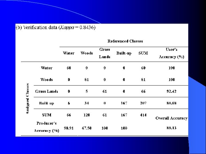
Gaussian-based maximum likelihood method

Indicator kriging method

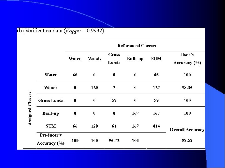
Although both classification methods result in very high overall accuracies, it is noteworthy that the indicator kriging classifier has significant superiority over the maximum likelihood classifier with regards to producer’s and user’s accuracies using verification data. For example, producer’s accuracy of woods is 67. 50% for the Gaussian-based maximum likelihood method, as compared to 100% for the indicator kriging method.

Scattering of the training data in twodimensional feature space

Scattering of the classified pixels by maximum likelihood method in twodimensional feature space

Scattering of the classified pixels by indicator kriging method in twodimensional feature space

Classification results of the Gaussianbased maximum likelihood method

Classification results of the indicator kriging method

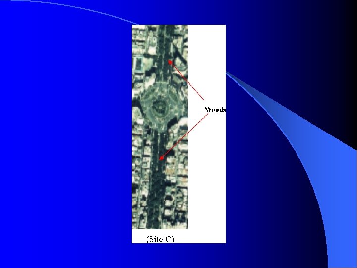
True color details of three exemplar sites (circled sites) demonstrate that Gaussianbased maximum likelihood method misclassifies woods to grass lands in site A and woods to built-up in sites B and C.

True color details of three exemplar sites