A Dynamic Optimal Capital Structure Model with Costly

A Dynamic Optimal Capital Structure Model with Costly Adjustment Mechanisms Hsien-Hsing, Liao Yi-Hsuan, Tung Tsung-kang Chen Department of Finance National Taiwan University 2008. 12

Abstract • In this study, we extend Goldstein, Ju and Leland (2001) to a cash flow-based model with costly adjustment mechanisms suggested by Leary and Roberts (2005) and include a fixed and a proportional cost elements in the mechanisms. • Main Results: ▫ Costs of capital structure adjustments, including a fixed cost element and a proportional one, have significant effect on the frequency and size of adjustments in capital structure by a firm. ▫ Our model is able to consider multiple types of adjustments, such as issuing and repurchasing either debt or equity. ▫ The numerical results of simulation analysis of our model are consistent with those expected in literature and intuition. 2

3 A Dynamic Optimal Capital Structure Model with Costly Adjustment Mechanisms Agenda • • • Introduction Description of the model Dynamic Capital Structure Strategy Numerical Results Conclusion

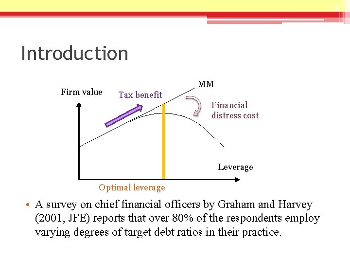
4 Introduction Firm value MM Tax benefit Financial distress cost Leverage Optimal leverage • A survey on chief financial officers by Graham and Harvey (2001, JFE) reports that over 80% of the respondents employ varying degrees of target debt ratios in their practice.

5 Introduction • There are substantial debates on the idea of a target debt ratio: ØFama and French (2002, RFS) suggest that firms seem slowly to rebalance their leverage to their long-run mean or optimal level. ØBaker and Wurgler (2002, JF) document that current capital structure is strongly related to historical market values and firm times equity issuances with high market valuations and has persistent effects on capital structure. ØWelch (2004, JPE) observes that stock price changes have a strong effect on market leverage ratios.

6 Introduction • Other literatures have disparate estimated results: ØFlannery and Rangan (2005, JFE) find that firms do target a long run capital structure and that a typical firm converges toward its long-run target at a rate of more than 30% per year. ØKayhan and Titman (2007, JFE) indicate that after controlling for the changes in stock prices and other timing and pecking order effects, changes in debt ratios are still partially explained by movements towards a target debt ratio.

7 Introduction • There are growing literature that considers adjustment costs to explain the relatively slow movement towards optimal leverage. ØFischer, Heinkel and Zechner (1989, JF) develop a model of dynamic capital structure choice in the presence of recapitalization costs. They find that even small recapitalization costs lead to wide swings in a firm's debt ratio over time.

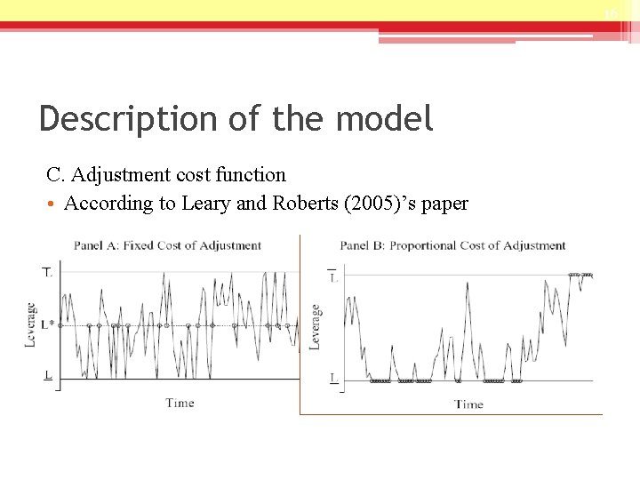
8 Introduction ØLeary and Roberts (2005, JF) shows that the presence of adjustment costs has significant implications for corporate financial policy. ◦ They reexamine the conclusions of Baker and Wurgler (2002, JF) and find that the persistence revealed by their empirical tests is more likely due to adjustment costs. ◦ They also find that the effect of Baker and Wurgler’s key market timing variable on leverage attenuates significantly as adjustment costs decline, proving that adjustment costs appear to dictate the speed at which firms respond to leverage shocks.

9 Introduction • These studies ignore the possibility that economic shocks may cause their optimal capital structure to change over time. • There are several theoretical dynamic capital structure models developed such as • Fischer, Heinkel and Zechner (1989, JF); • Goldstein, Ju, and Leland (2001, JB); • Titman and Tsyplakov (2007, wp).

10 Introduction • Based on Goldstein, Ju, and Leland (2001, JB), we develop a dynamic capital structure model that allows us to determine the value of firm, value of debt, value of bankruptcy, optimal coupon and leverage endogenously, and to quantify the benefits and costs associated with both movements towards and away from optimal capital structure.

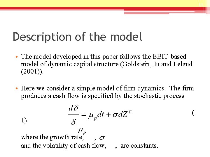
11 Description of the model • The model developed in this paper follows the EBIT-based model of dynamic capital structure (Goldstein, Ju and Leland (2001)). • Here we consider a simple model of firm dynamics. The firm produces a cash flow is specified by the stochastic process ( 1) where the growth rate, , and the volatility of cash flow, , are constants.

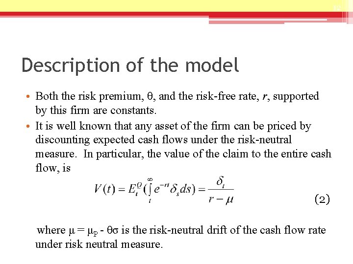
12 Description of the model • Both the risk premium, θ, and the risk-free rate, r, supported by this firm are constants. • It is well known that any asset of the firm can be priced by discounting expected cash flows under the risk-neutral measure. In particular, the value of the claim to the entire cash flow, is (2) where μ = μP - θσ is the risk-neutral drift of the cash flow rate under risk neutral measure.

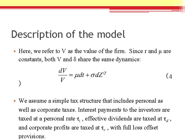
13 Description of the model • Here, we refer to V as the value of the firm. Since r and μ are constants, both V and δ share the same dynamics: (4 ) • We assume a simple tax structure that includes personal as well as corporate taxes. Interest payments to the investors are taxed at a personal rate τi , effective dividends are taxed at τd , and corporate profits are taxed at τc , with full loss offset provisions.

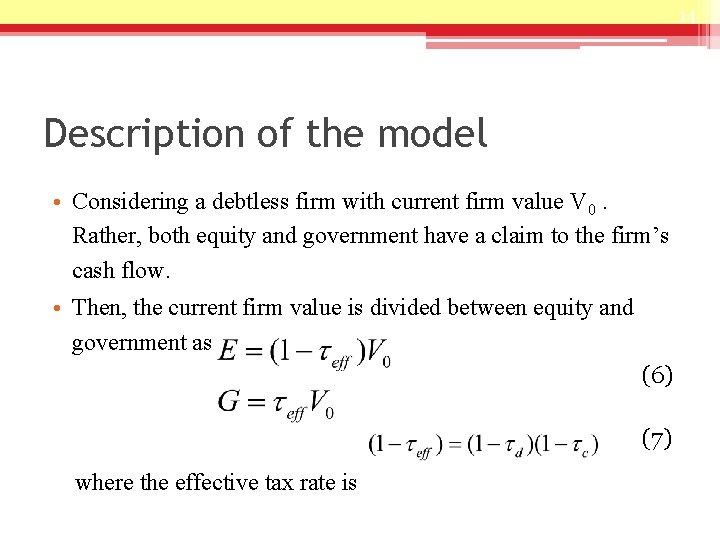
14 Description of the model • Considering a debtless firm with current firm value V 0. Rather, both equity and government have a claim to the firm’s cash flow. • Then, the current firm value is divided between equity and government as (6) (7) where the effective tax rate is

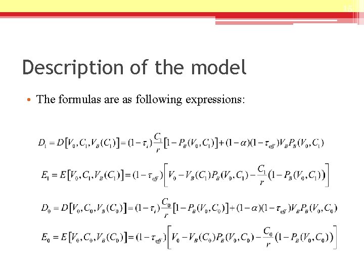
15 Description of the model • The formulas are as following expressions:

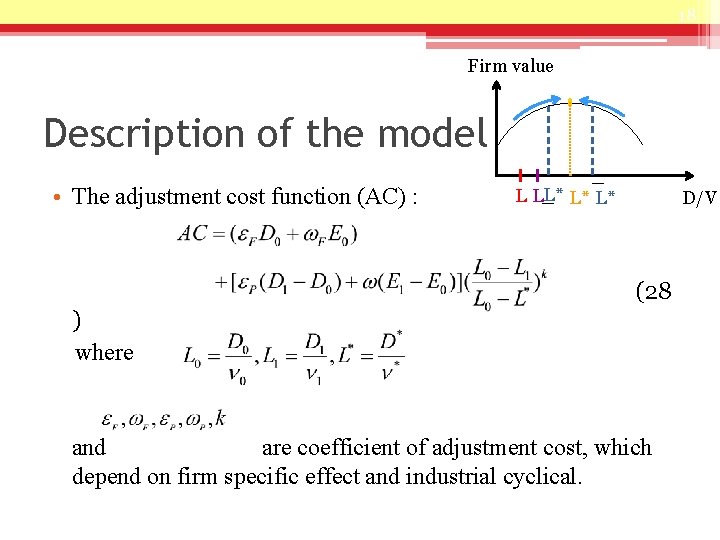
16 Description of the model C. Adjustment cost function • According to Leary and Roberts (2005)’s paper

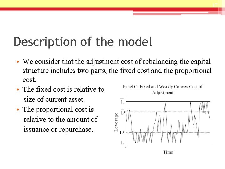
17 Description of the model • We consider that the adjustment cost of rebalancing the capital structure includes two parts, the fixed cost and the proportional cost. • The fixed cost is relative to size of current asset. • The proportional cost is relative to the amount of issuance or repurchase.

18 Firm value Description of the model • The adjustment cost function (AC) : L LL* L* L* D/V (28 ) where and are coefficient of adjustment cost, which depend on firm specific effect and industrial cyclical.

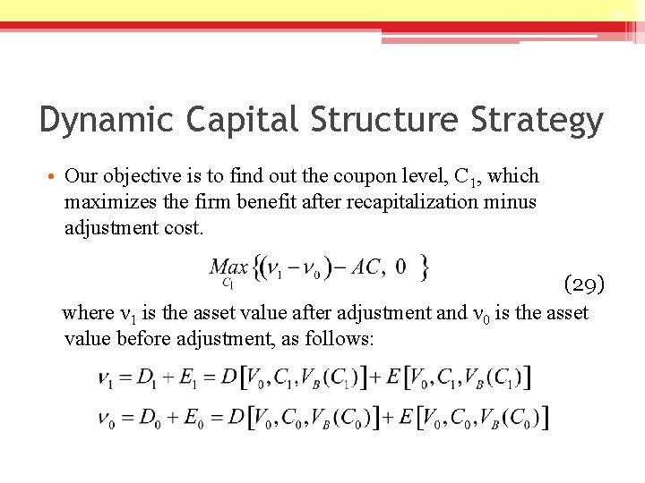
19 Dynamic Capital Structure Strategy • Our objective is to find out the coupon level, C 1, which maximizes the firm benefit after recapitalization minus adjustment cost. (29) where ν 1 is the asset value after adjustment and ν 0 is the asset value before adjustment, as follows:

20 Dynamic Capital Structure Strategy • There are two situations that we choose to recapitalize: 1. When the firm value touch to the default value. 2. When the benefit of recapitalization is larger than cost. • We calculate the firm value, V (eq. [2]), and determine whether it is larger than the bankruptcy level, VB, at each period. ◦ If V<VB, adjust to optimal coupon level. (eq. [27]) ◦ If V>VB, adjust to coupon level C 1. (eq. [29])

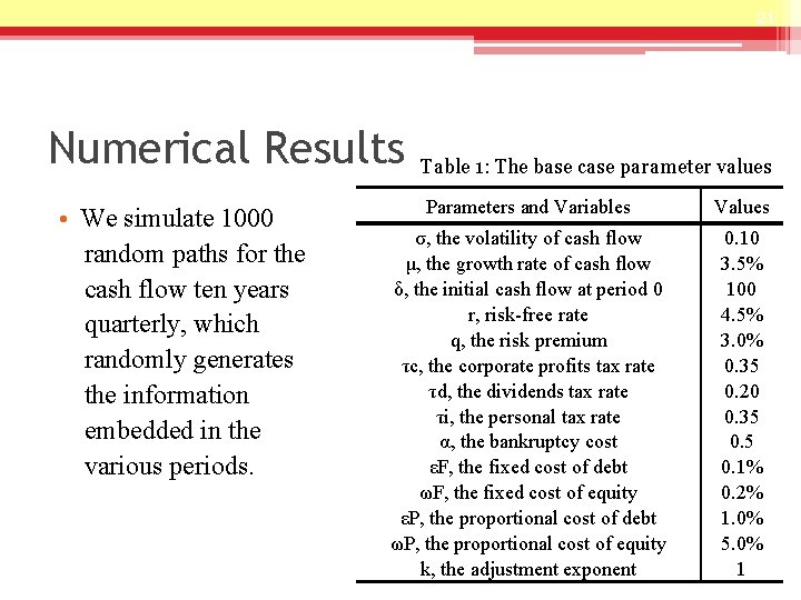
21 Numerical Results • We simulate 1000 random paths for the cash flow ten years quarterly, which randomly generates the information embedded in the various periods. Table 1: The base case parameter values Parameters and Variables Values σ, the volatility of cash flow μ, the growth rate of cash flow δ, the initial cash flow at period 0 r, risk-free rate q, the risk premium τc, the corporate profits tax rate τd, the dividends tax rate τi, the personal tax rate α, the bankruptcy cost εF, the fixed cost of debt ωF, the fixed cost of equity εP, the proportional cost of debt ωP, the proportional cost of equity k, the adjustment exponent 0. 10 3. 5% 100 4. 5% 3. 0% 0. 35 0. 20 0. 35 0. 1% 0. 2% 1. 0% 5. 0% 1

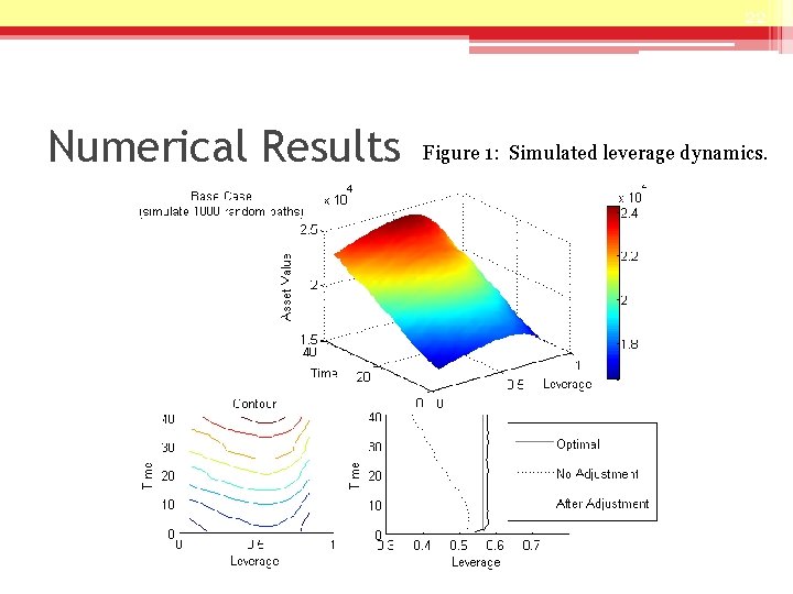
22 Numerical Results Figure 1: Simulated leverage dynamics.

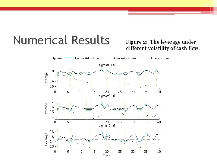
23 Numerical Results Figure 2: The leverage under different volatility of cash flow.

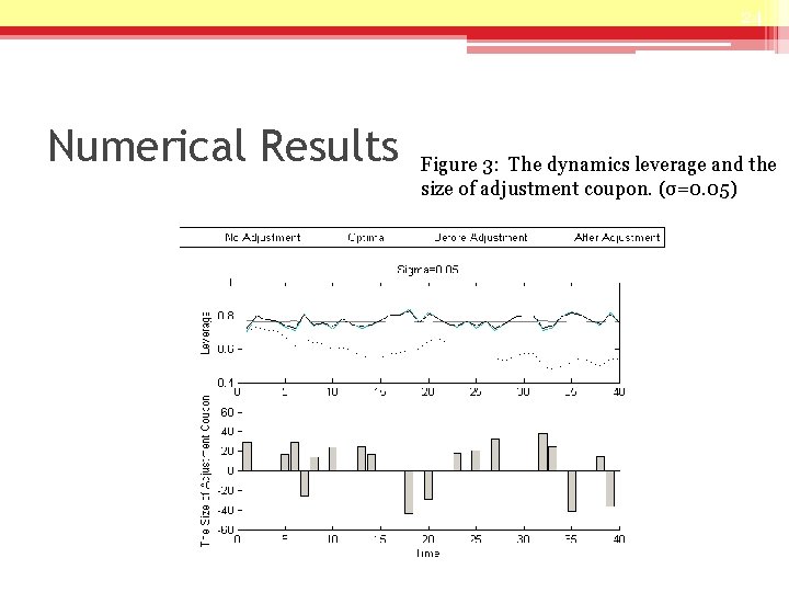
24 Numerical Results Figure 3: The dynamics leverage and the size of adjustment coupon. (σ=0. 05)

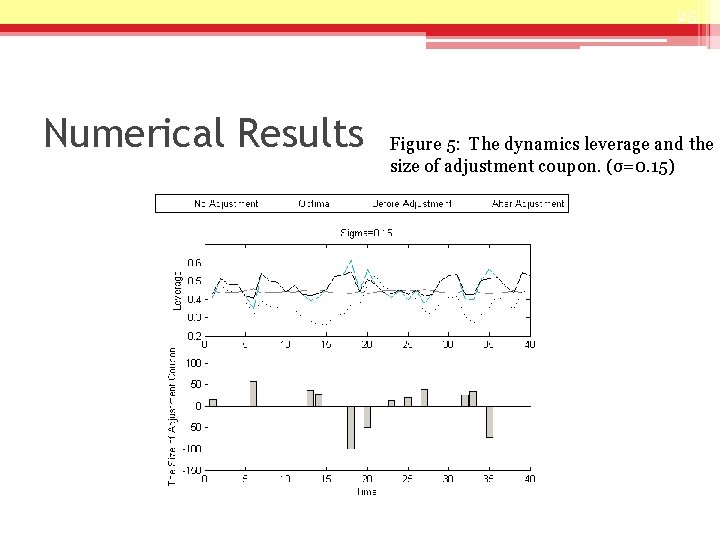
25 Numerical Results Figure 5: The dynamics leverage and the size of adjustment coupon. (σ=0. 15)

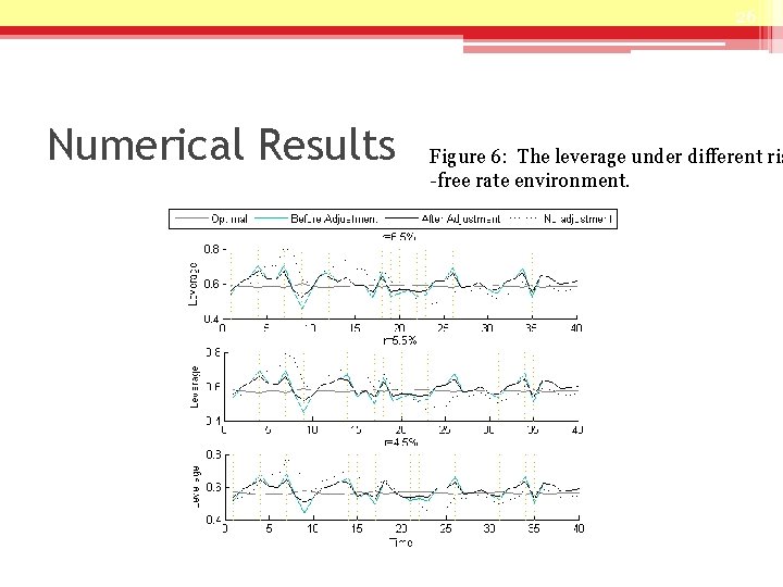
26 Numerical Results Figure 6: The leverage under different ris -free rate environment.

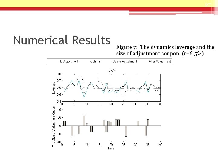
27 Numerical Results Figure 7: The dynamics leverage and the size of adjustment coupon. (r=6. 5%)

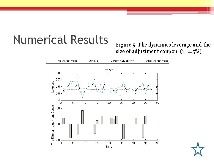
28 Numerical Results Figure 9 The dynamics leverage and the size of adjustment coupon. (r=4. 5%)

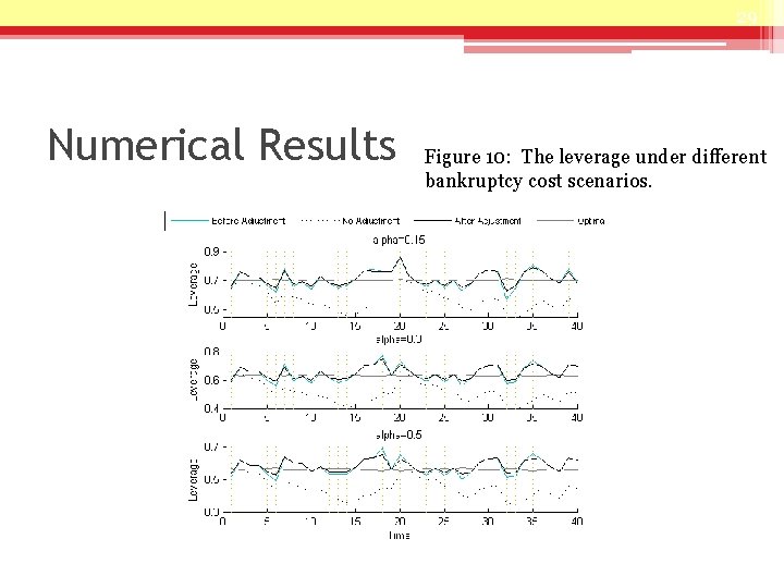
29 Numerical Results Figure 10: The leverage under different bankruptcy cost scenarios.

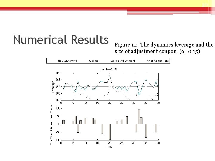
30 Numerical Results Figure 11: The dynamics leverage and the size of adjustment coupon. (α=0. 15)

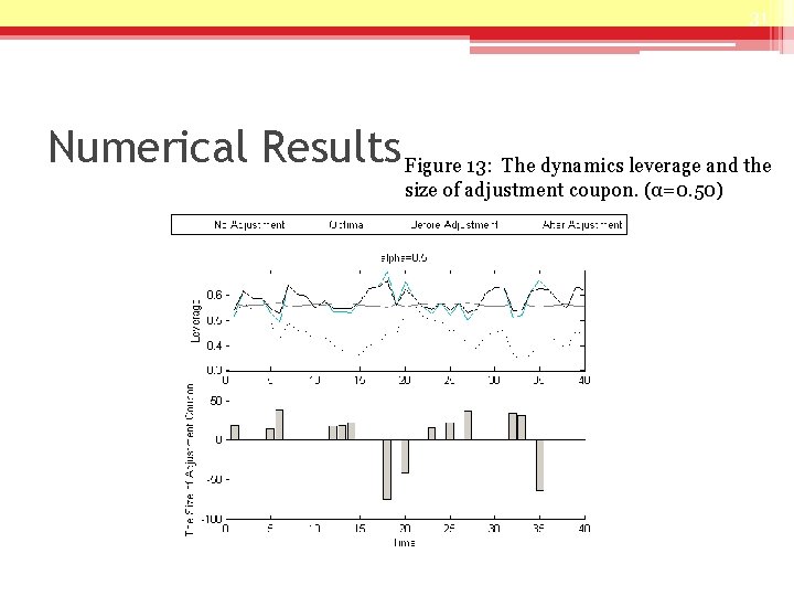
31 Numerical Results Figure 13: The dynamics leverage and the size of adjustment coupon. (α=0. 50)

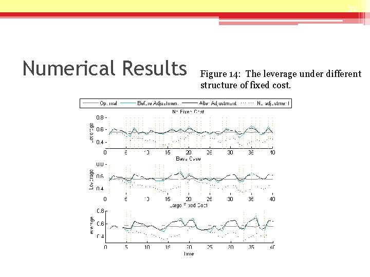
32 Numerical Results Figure 14: The leverage under different structure of fixed cost.

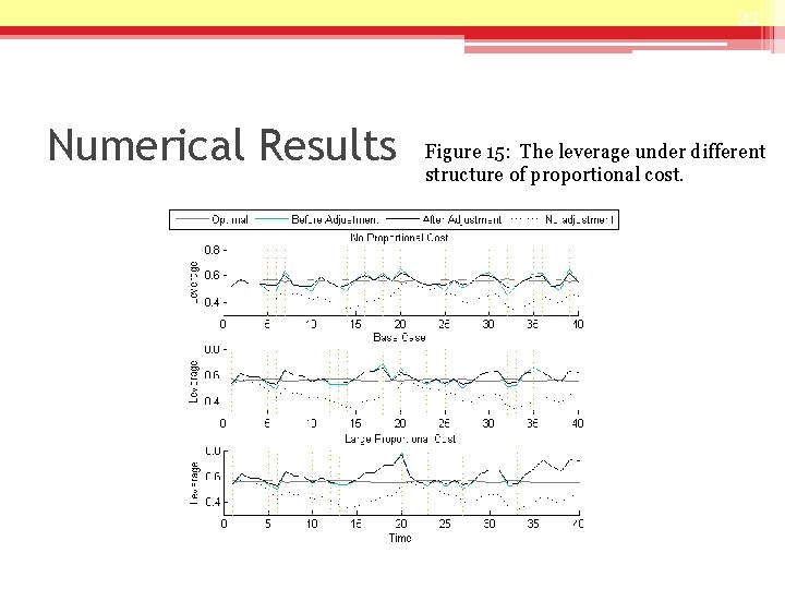
33 Numerical Results Figure 15: The leverage under different structure of proportional cost.

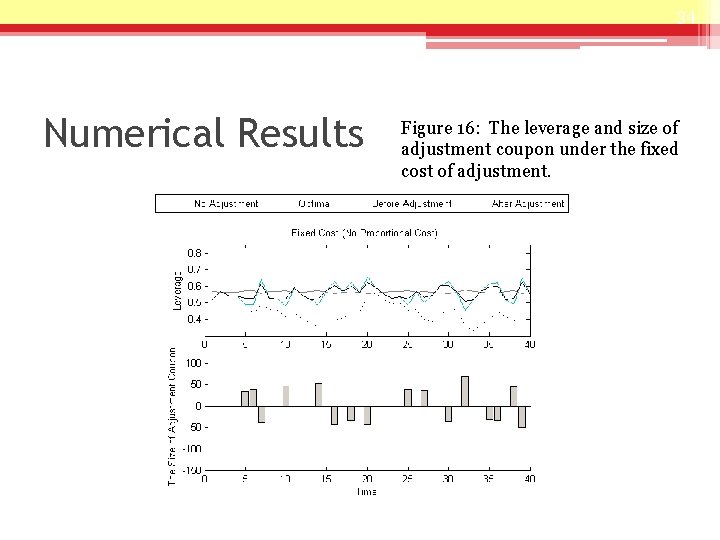
34 Numerical Results Figure 16: The leverage and size of adjustment coupon under the fixed cost of adjustment.

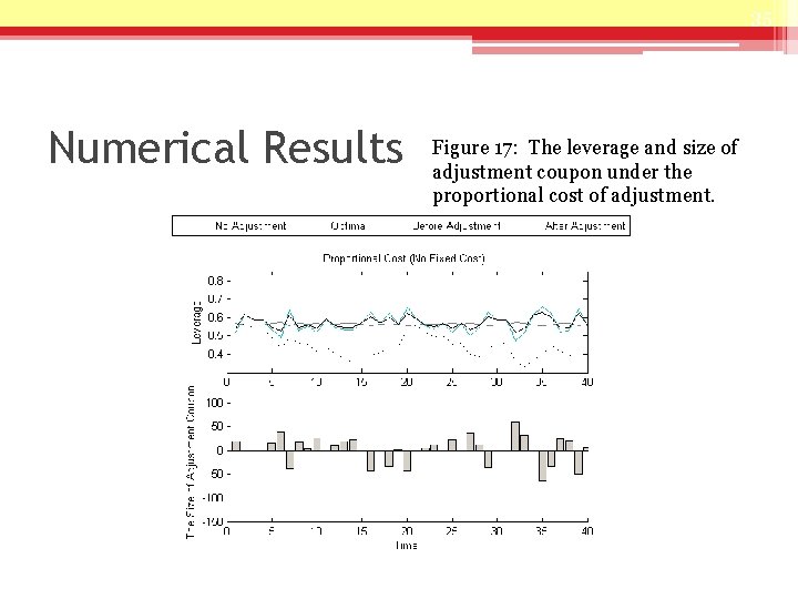
35 Numerical Results Figure 17: The leverage and size of adjustment coupon under the proportional cost of adjustment.

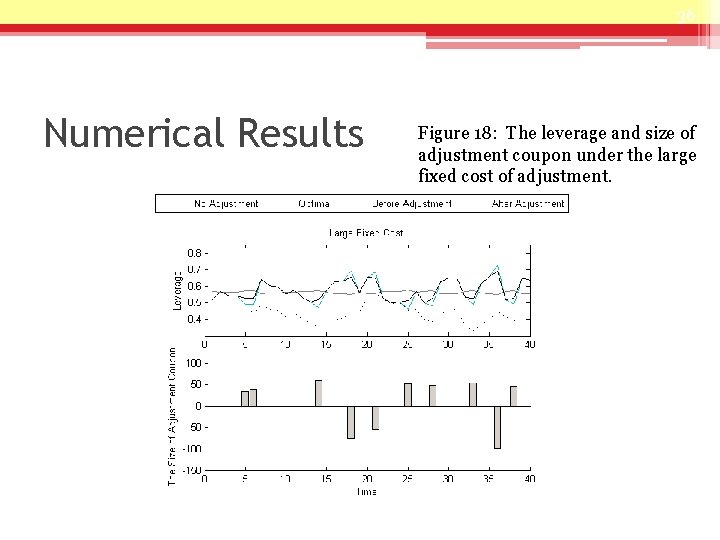
36 Numerical Results Figure 18: The leverage and size of adjustment coupon under the large fixed cost of adjustment.

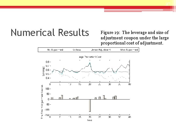
37 Numerical Results Figure 19: The leverage and size of adjustment coupon under the large proportional cost of adjustment.

38 Conclusion • We modify a EBIT-based Model proposed by Goldstein, Ju, and Leland(2001), and develop dynamic capital structure model with costly adjustment mechanisms. • We consider costs of capital adjustments, including a fixed cost element and a proportional one, which have significant effect on the frequency and size of adjustments in capital structure by a firm. • Our model is able to consider multiple types of adjustments, such as issuing and repurchasing either debt or equity.

39 Conclusion • Based on an exogenous cash flow process, the model can endogenously determine the firm value and the claim value of firm’s derivative security under optimal debt level. • A firm can alter the variables of the model based on industry and firm specific properties to determine if doing a recapitalization at any point in time. • Finally, the numerical results of simulation analysis of our model are consistent with those expected in literature and intuition.

40 Reference [1] Baker, Malcolm, and Jeffrey Wurgler, 2002, “Market timing and capital structure”, Journal of Finance 57, 1– 30. [2] Fama, E. F. and K. R. French, 2002, “Testing trade-off and pecking order predictions about dividends and debt”, The Review of Financial Studies 15(1): 1 -33. [3] Fischer, E. , Heinkel, R. , and J. Zechner, 1989 a, “Dynamic Capital Structure Choice: Theory and Tests”, Journal of Finance 44, 19 -40. [4] Flannery M. and K. Rangan, 2006, “Partial Adjustment toward Target Capital Structures”, Journal of Financial Economics 79, 469 -506. [5] Goldstein, R. , Ju, N. , and H. Leland, 2001, “ An EBIT Based Model of Dynamic Capital Structure”, Journal of Business 74, 483 -512. [6] Graham, J. , and Harvey C. , 2001, “The Theory and Practice of Corporate Finance: Evidence from the Field”, Journal of Financial Economics 60, 187 -243. [7] Hovakimian, A. , Opler T, and S. Titman, 2001, “The Debt-Equity Choice”, Journal of Financial And Quantitative Analysis, 36 (1), 1 -24. [8] Kayhan A, . and S. Titman, 2007, “ Firms’ Histories and Their Capital Structure”, Journal of Financial Economics 83, 1 -32.

41 Reference [9] Leary M. , and M. Roberts, 2005, “Do Firms Rebalance Their Capital Structures? ”, Journal of Finance , 2575 -2619. [10] Leland, H. E. , 1994, “Corporate Debt Value, Bond Covenants, and Optimal Capital Structure”, Journal of Finance, 1213 -1252. [11] Leland, H. E. and K. B. , Toft, 1996, “Optimal Capital Structure, Endogenous Bankruptcy, and the Term Structure of Credit Spreads”, Journal of Finance 51, 987 -1019. [12] Leland, H. E. , 1998, “Agency Costs, Risk Management, and Capital Structure”, Journal of Finance 53, 1213 -1243. [13] Miller, M. H. 1977 “Debt and Taxes, ” Journal of Finance 32, No. 2, 261 -275. [14] Modigliani, Franco, and Merton H. Miller, 1963, “Corporate income taxes and the cost of capital: A correction”, American Economic Review, 53, 433 -443. [15] Sheridan Titman and Sergey Tsyplakov, 2007, “A Dynamic Model of Optimal Capital Structure”, working paper. [16] Welch, Ivo, 2004, “Capital structure and stock returns”, Journal of Political Economy 112, 106– 131.

42 Description of the model • Consider an otherwise identical firm whose management decides to choose a static leverage level that will maximize the wealth of current equity holders. • We assume a firm will issue a perpetual bond, promising a constant coupon payment C to debt holders as long as the firm remains solvent. • We define the firm chooses the default threshold as VB. If the firm value reaches VB , then an amount αVB will be lost due to bankruptcy costs. 42

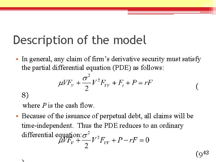
43 Description of the model • In general, any claim of firm’s derivative security must satisfy the partial differential equation (PDE) as follows: ( 8) where P is the cash flow. • Because of the issuance of perpetual debt, all claims will be time-independent. Thus the PDE reduces to an ordinary differential equation: (943

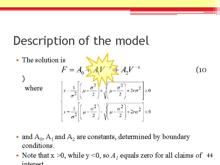
44 Description of the model • The solution is (10 ) where • and A 0, A 1 and A 2 are constants, determined by boundary conditions. • Note that x >0, while y <0, so A 1 equals zero for all claims of 44

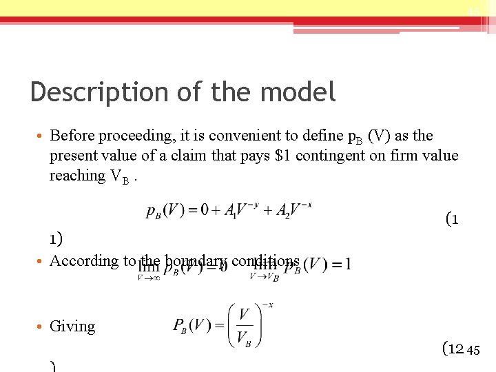
45 Description of the model • Before proceeding, it is convenient to define p. B (V) as the present value of a claim that pays $1 contingent on firm value reaching VB. (1 1) • According to the boundary conditions • Giving (12 45

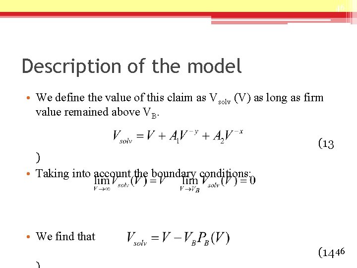
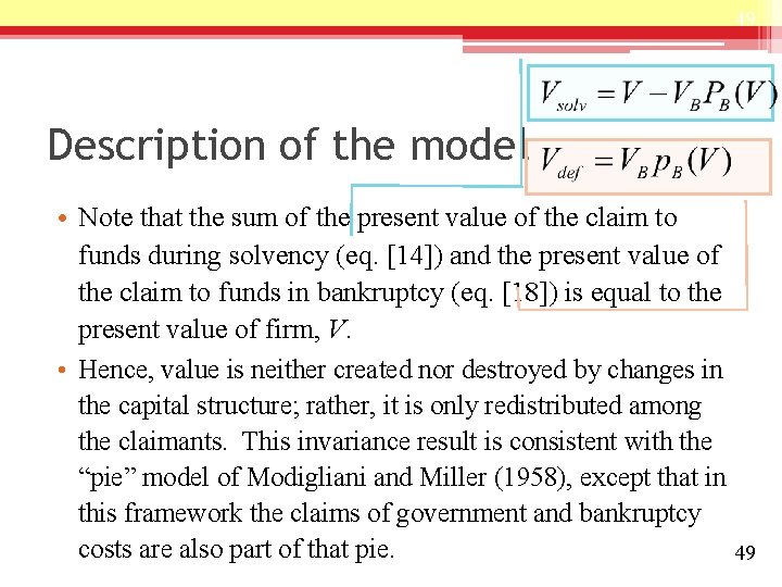
46 Description of the model • We define the value of this claim as Vsolv (V) as long as firm value remained above VB. (13 ) • Taking into account the boundary conditions: • We find that (14 46

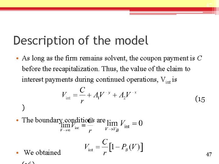
47 Description of the model • As long as the firm remains solvent, the coupon payment is C before the recapitalization. Thus, the value of the claim to interest payments during continued operations, Vint is (15 ) • The boundary conditions are • We obtained 47

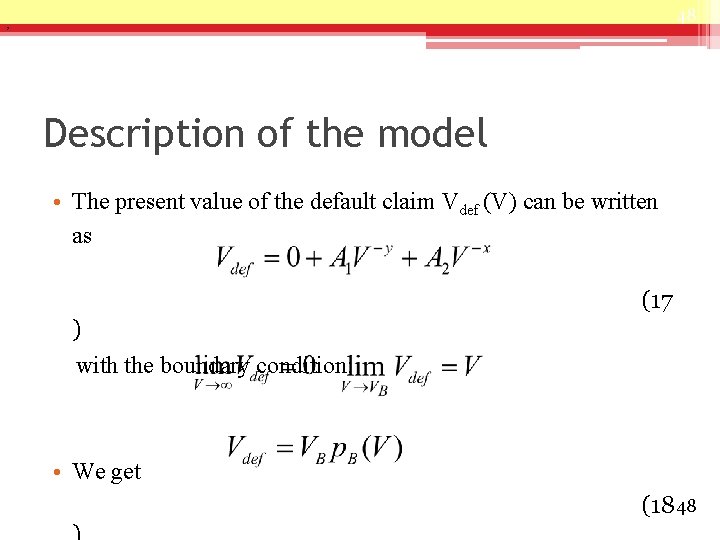
48 , Description of the model • The present value of the default claim Vdef (V) can be written as (17 ) with the boundary condition: • We get (1848

49 Description of the model • Note that the sum of the present value of the claim to funds during solvency (eq. [14]) and the present value of the claim to funds in bankruptcy (eq. [18]) is equal to the present value of firm, V. • Hence, value is neither created nor destroyed by changes in the capital structure; rather, it is only redistributed among the claimants. This invariance result is consistent with the “pie” model of Modigliani and Miller (1958), except that in this framework the claims of government and bankruptcy costs are also part of that pie. 49

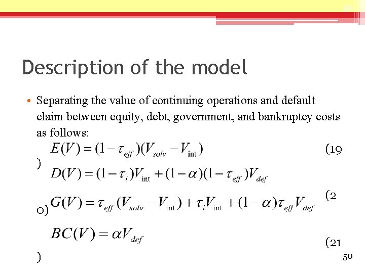
50 Description of the model • Separating the value of continuing operations and default claim between equity, debt, government, and bankruptcy costs as follows: (19 ) (2 0) (21 ) 50

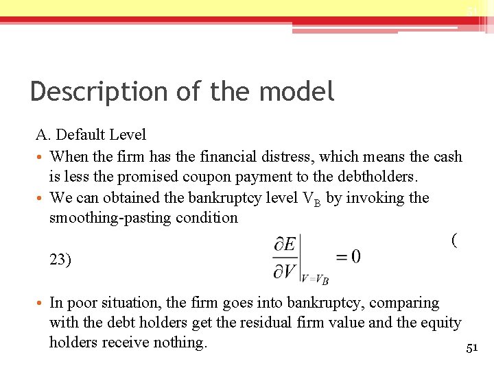
51 Description of the model A. Default Level • When the firm has the financial distress, which means the cash is less the promised coupon payment to the debtholders. • We can obtained the bankruptcy level VB by invoking the smoothing-pasting condition ( 23) • In poor situation, the firm goes into bankruptcy, comparing with the debt holders get the residual firm value and the equity holders receive nothing. 51

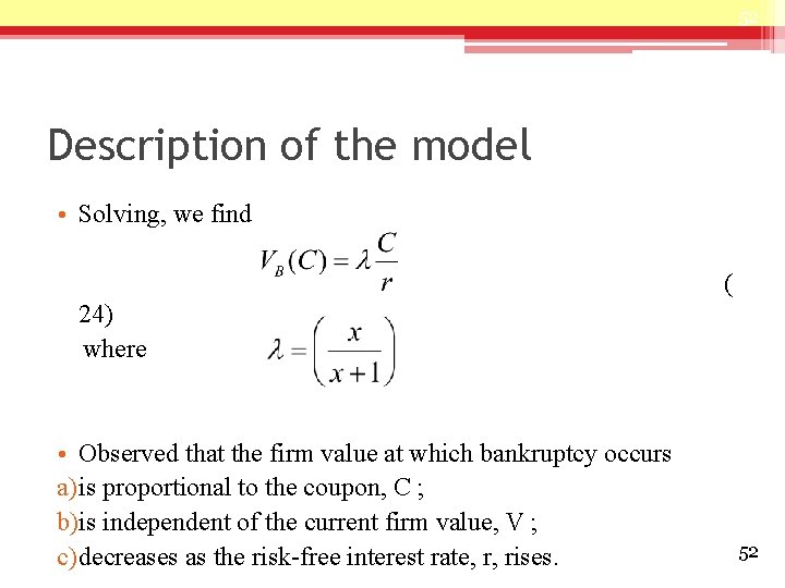
52 Description of the model • Solving, we find ( 24) where • Observed that the firm value at which bankruptcy occurs a) is proportional to the coupon, C ; b)is independent of the current firm value, V ; c) decreases as the risk-free interest rate, r, rises. 52

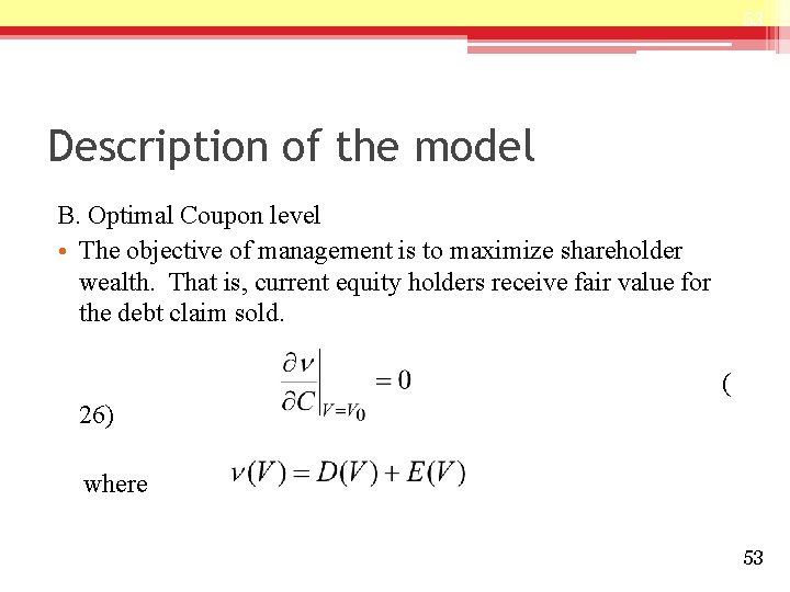
53 Description of the model B. Optimal Coupon level • The objective of management is to maximize shareholder wealth. That is, current equity holders receive fair value for the debt claim sold. ( 26) where 53

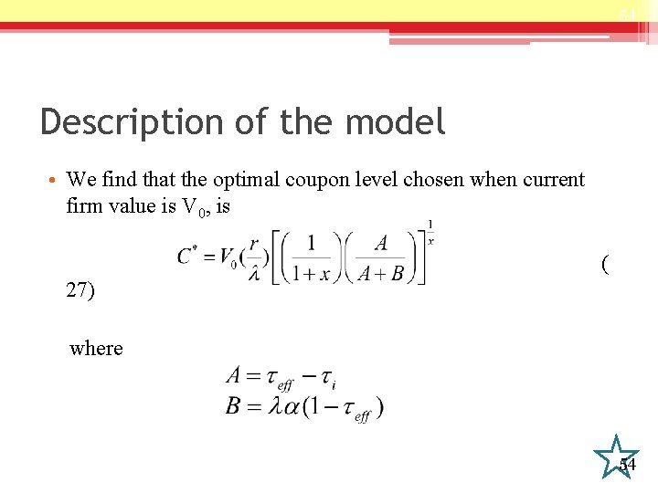
54 Description of the model • We find that the optimal coupon level chosen when current firm value is V 0, is ( 27) where 54