A Dynamic Mobility Histogram Construction Method Based on

A Dynamic Mobility Histogram Construction Method Based on Markov Chains Yoshiharu Ishikawa (Nagoya University) Yoji Machida (University of Tsukuba) Hiroyuki Kitagawa (University of Tsukuba)

Outline • • • Background and Objectives Modeling Movement Patterns Mobility Histogram: Logical Structure Mobility Histogram: Physical Structure Experimental Results Conclusions 1
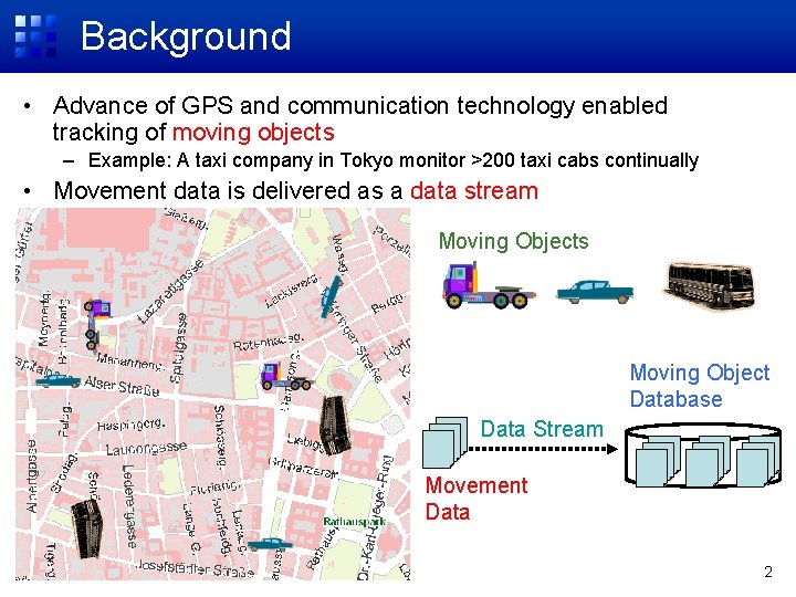
Background • Advance of GPS and communication technology enabled tracking of moving objects – Example: A taxi company in Tokyo monitor >200 taxi cabs continually • Movement data is delivered as a data stream Moving Objects Moving Object Database Data Stream Movement Data 2

Objectives • Construction and maintenance of a mobility histogram – Compact summary of movement data for a specific time period – Used for mobility analysis and estimation • Problems – Concrete definition of a mobility histogram • How to model movement patterns – Compact representation • Tradeoff with accuracy – Efficient construction and maintenance • Incremental processing for streamed data 3
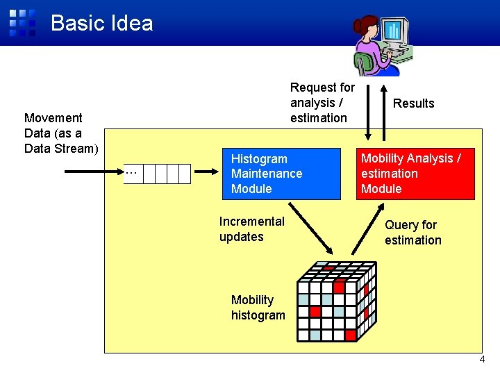
Basic Idea Request for analysis / estimation Movement Data (as a Data Stream) … Histogram Maintenance Module Incremental updates Results Mobility Analysis / estimation Module Query for estimation Mobility histogram 4
Outline • • • Background and Objectives Modeling Movement Patterns Mobility Histogram: Logical Structure Mobility Histogram: Physical Structure Experimental Results Conclusions 5
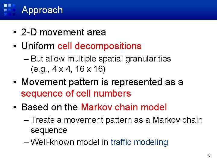
Approach • 2 -D movement area • Uniform cell decompositions – But allow multiple spatial granularities (e. g. , 4 x 4, 16 x 16) • Movement pattern is represented as a sequence of cell numbers • Based on the Markov chain model – Treats a movement pattern as a Markov chain sequence – Well-known model in traffic modeling 6
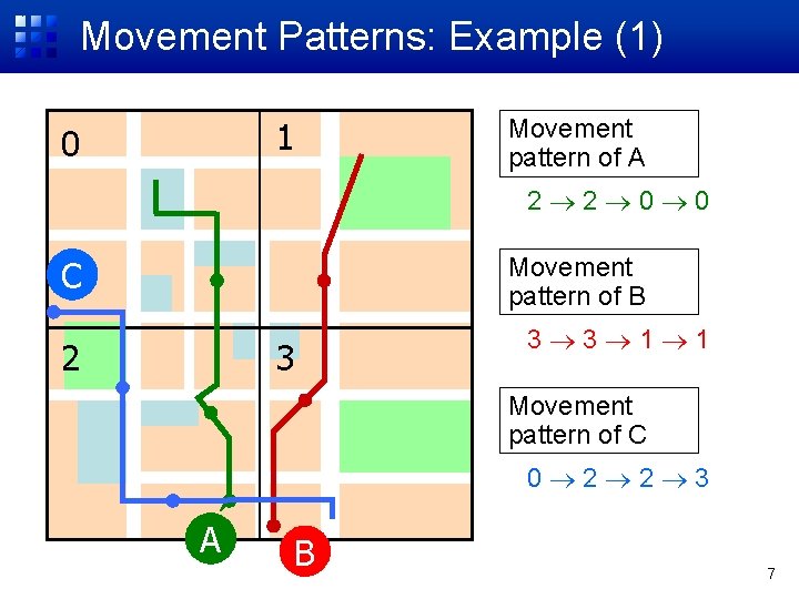
Movement Patterns: Example (1) 1 0 Movement pattern of A 2 2 0 0 Movement pattern of B C 2 3 3 3 1 1 Movement pattern of C 0 2 2 3 A B 7
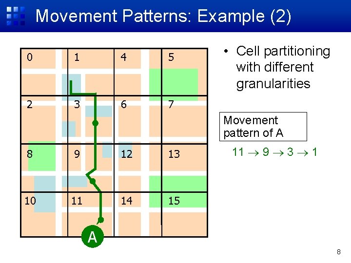
Movement Patterns: Example (2) 0 1 4 5 2 3 6 7 • Cell partitioning with different granularities Movement pattern of A 8 9 12 13 10 11 14 15 11 9 3 1 A 8
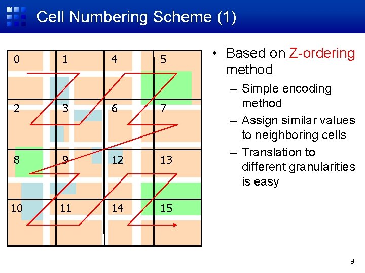
Cell Numbering Scheme (1) 0 1 4 5 2 3 6 7 8 9 12 13 10 11 14 15 • Based on Z-ordering method – Simple encoding method – Assign similar values to neighboring cells – Translation to different granularities is easy 9
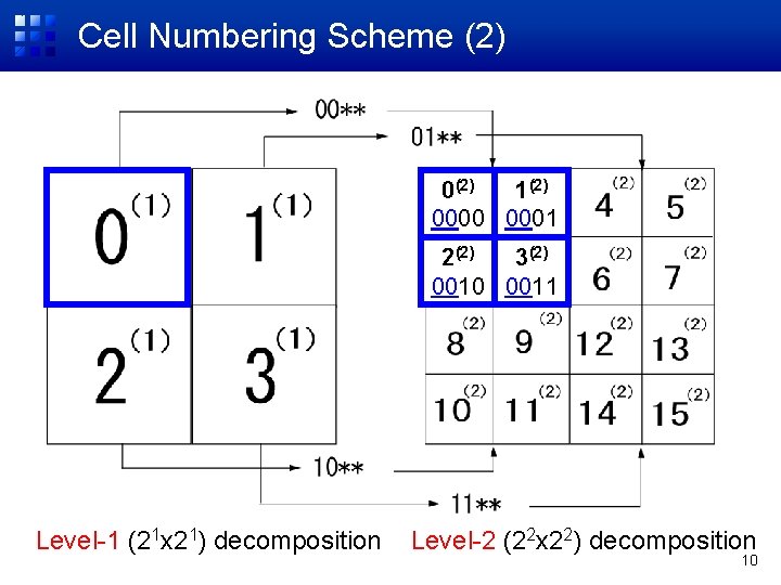
Cell Numbering Scheme (2) 0(2) 1(2) 0000 0001 2(2) 3(2) 0010 0011 Level-1 (21 x 21) decomposition Level-2 (22 x 22) decomposition 10
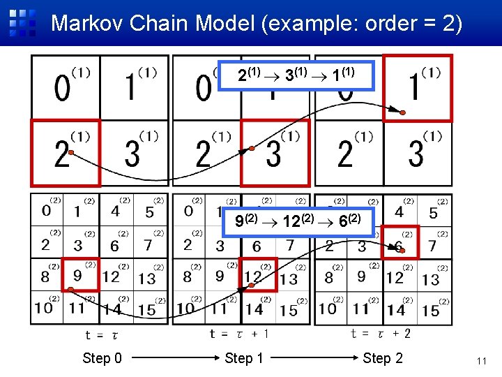
Markov Chain Model (example: order = 2) 2(1) 3(1) 1(1) 9(2) 12(2) 6(2) Step 0 Step 1 Step 2 11
Outline • • • Background and Objectives Modeling Movement Patterns Mobility Histogram: Logical Structure Mobility Histogram: Physical Structure Experimental Results Conclusions 12
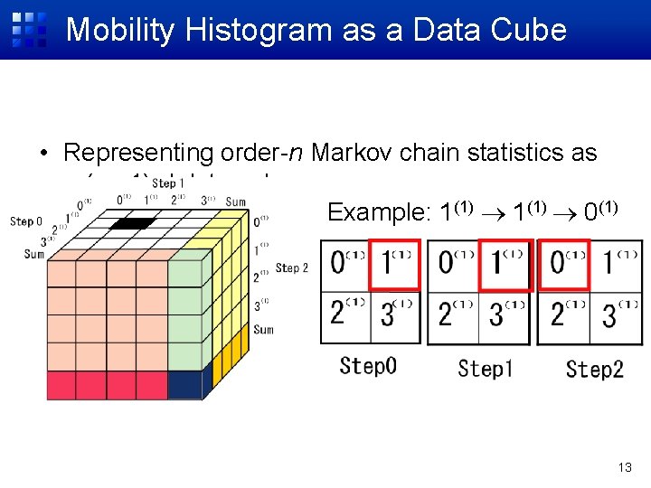
Mobility Histogram as a Data Cube • Representing order-n Markov chain statistics as a (n +1)-d data cube Example: 1(1) 0(1) 13

Histogram Maintenance Movement Data … Histogram Maintenance Module Incremental updates Mobility Analysis / Estimation Module Query for analysis Mobility histogram … • Periodical reconstruction – To cope with non-stationary movement patterns – Ease of maintenance – Old histograms are written to disk 14
Outline • • • Background and Objectives Modeling Movement Patterns Mobility Histogram: Logical Structure Mobility Histogram: Physical Structure Experimental Results Conclusions 15
Mobility Histogram: Physical Structure • Problems in logical structure: huge space – 2 GB (!) for a typical parameter setting – Needs multiple cubes for multiple spatial granularities – Data cubes are sparse: most of mobility patterns are hard to occur • Solution: tree-based representation – Unification of quad-tree, k-d tree, and trie – Integration of cubes in multiple granularities – Selective allocation of nodes • Saves memory space 16
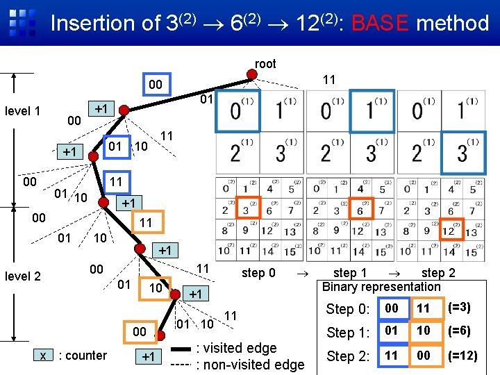
Insertion of 3(2) 6(2) 12(2): BASE method root 11 00 level 1 00 11 01 10 +1 00 11 01 level 2 11 01 10 +1 00 01 +1 10 +1 11 00 01 10 00 x : counter +1 step 0 +1 01 10 11 : visited edge : non-visited edge step 1 step 2 Binary representation Step 0: 00 11 (=3) Step 1: 01 10 (=6) Step 2: 11 00 (=12)
Approximated Histogram (APR) • Problem of the BASE method – Memory size requirement is still high • Approximated method (APR) – Compact histogram construction by adaptive tree expansion • Allocate a buffer for each leaf node • If skew is observed, the leaf node is expanded • 2 statistics is used to check the non-uniformity – Inherited the idea from decision tree construction from streamed data (e. g. , VFDT) 18
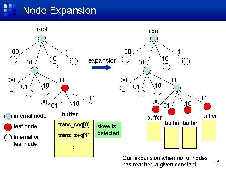
Node Expansion root 00 11 10 01 00 11 10 00 internal node expansion 11 00 01 01 10 11 internal or leaf node trans_seq[1] buffer skew is detected 01 10 11 buffer … trans_seq[0] 11 10 00 buffer leaf node 10 01 Quit expansion when no. of nodes has reached a given constant 19
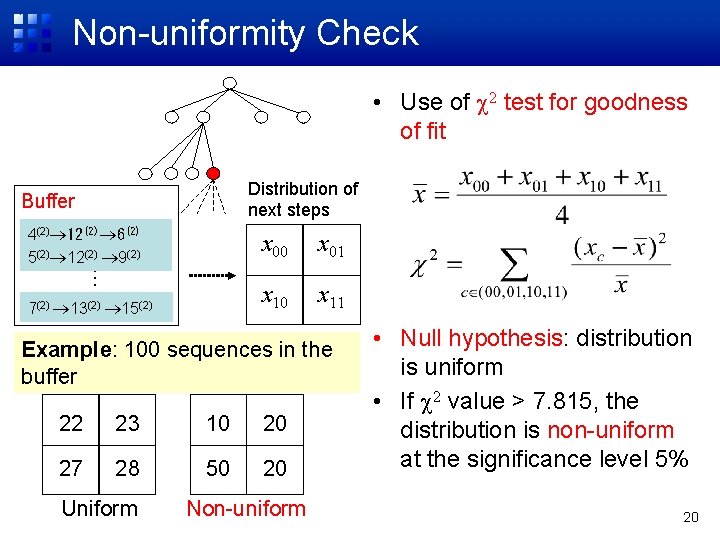
Non-uniformity Check • Use of 2 test for goodness of fit Distribution of next steps Buffer 4(2) 12(2) 6(2) 5(2) 12(2) 9(2) … 7(2) 13(2) 15(2) x 00 x 01 x 10 x 11 Example: 100 sequences in the buffer 22 23 10 20 27 28 50 20 Uniform Non-uniform • Null hypothesis: distribution is uniform • If 2 value > 7. 815, the distribution is non-uniform at the significance level 5% 20
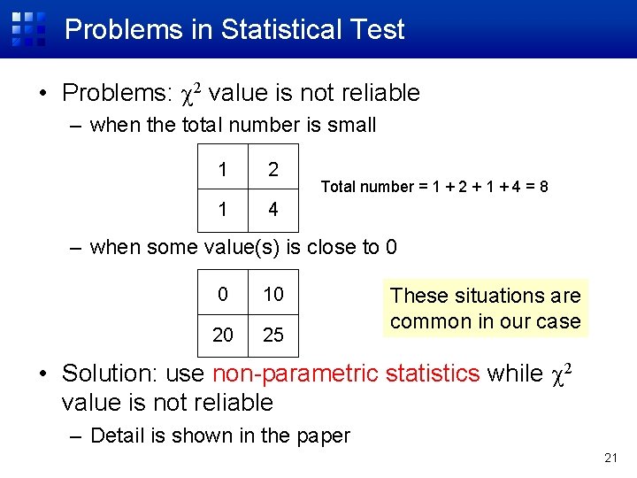
Problems in Statistical Test • Problems: 2 value is not reliable – when the total number is small 1 2 1 4 Total number = 1 + 2 + 1 + 4 = 8 – when some value(s) is close to 0 0 10 20 25 These situations are common in our case • Solution: use non-parametric statistics while 2 value is not reliable – Detail is shown in the paper 21
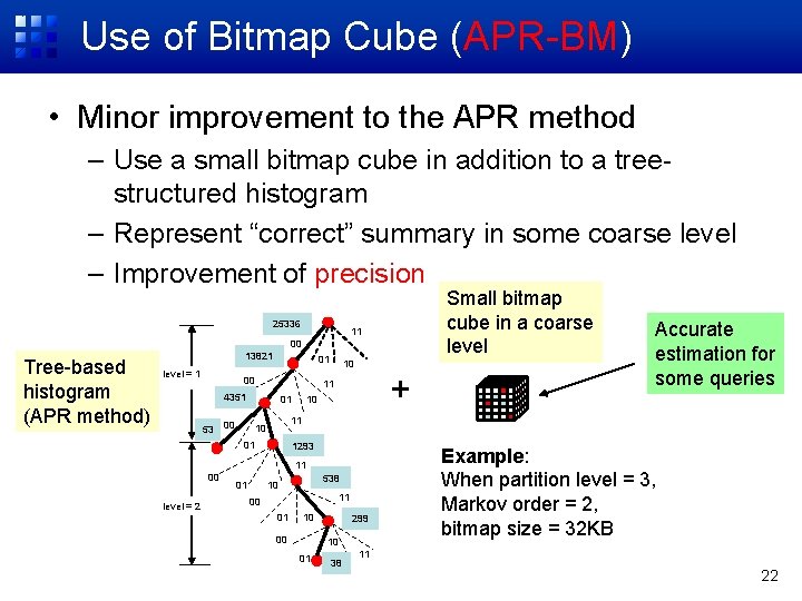
Use of Bitmap Cube (APR-BM) • Minor improvement to the APR method – Use a small bitmap cube in addition to a treestructured histogram – Represent “correct” summary in some coarse level – Improvement of precision 25336 Small bitmap cube in a coarse level 11 00 Tree-based histogram (APR method) 13821 level = 1 01 00 + 11 4351 53 10 10 11 10 01 1293 11 00 level = 2 01 Accurate estimation for some queries 538 10 11 00 01 10 00 299 10 01 38 Example: When partition level = 3, Markov order = 2, bitmap size = 32 KB 11 22
Outline • • • Background and Objectives Modeling Movement Patterns Mobility Histogram: Logical Structure Mobility Histogram: Physical Structure Experimental Results Conclusions 23
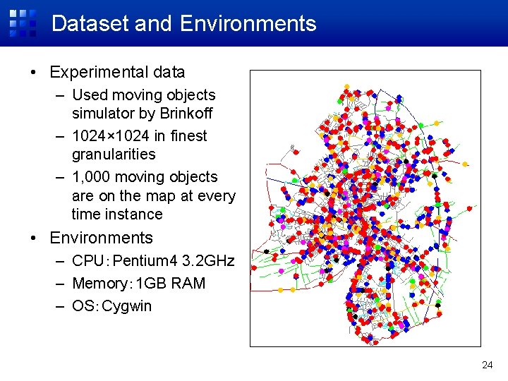
Dataset and Environments • Experimental data – Used moving objects simulator by Brinkoff – 1024× 1024 in finest granularities – 1, 000 moving objects are on the map at every time instance • Environments – CPU:Pentium 4 3. 2 GHz – Memory: 1 GB RAM – OS:Cygwin 24
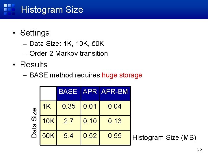
Histogram Size • Settings – Data Size: 1 K, 10 K, 50 K – Order-2 Markov transition • Results – BASE method requires huge storage Data Size BASE APR-BM 1 K 0. 35 0. 01 0. 04 10 K 2. 7 0. 10 0. 13 50 K 9. 4 0. 52 0. 55 Histogram Size (MB) 25
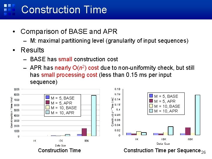
Construction Time • Comparison of BASE and APR – M: maximal partitioning level (granularity of input sequences) • Results – BASE has small construction cost – APR has nearly O(n 2) cost due to non-uniformity check, but still has small processing cost (less than 0. 15 ms per input sequence) M = 5, BASE M = 5, APR M = 10, BASE M = 10, APR Construction Time per Sequence 26
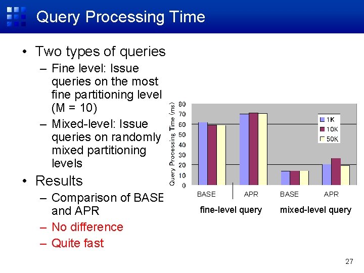
Query Processing Time • Two types of queries – Fine level: Issue queries on the most fine partitioning level (M = 10) – Mixed-level: Issue queries on randomly mixed partitioning levels • Results – Comparison of BASE and APR – No difference – Quite fast BASE APR fine-level query BASE APR mixed-level query 27
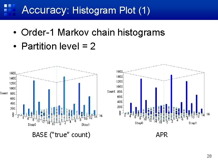
Accuracy: Histogram Plot (1) • Order-1 Markov chain histograms • Partition level = 2 BASE (“true” count) APR 28
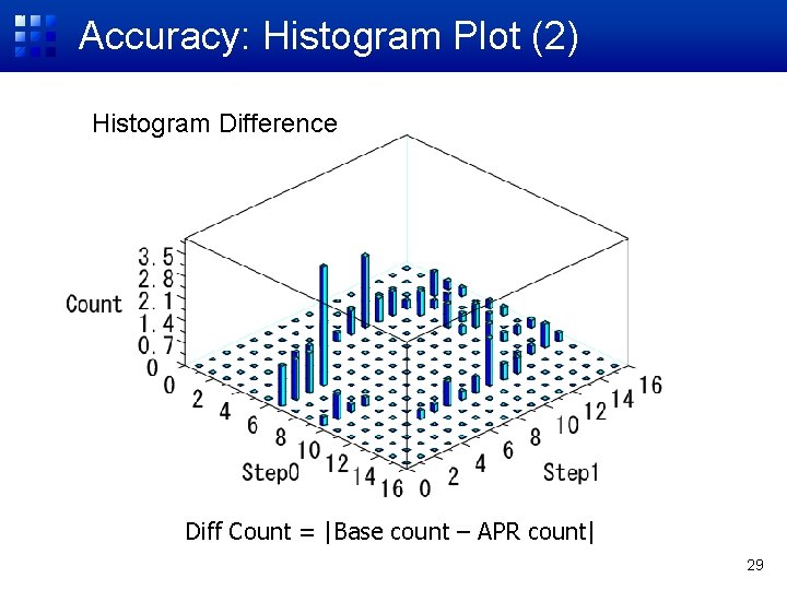
Accuracy: Histogram Plot (2) Histogram Difference Diff Count = |Base count – APR count| 29
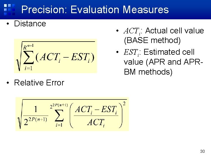
Precision: Evaluation Measures • Distance • ACTi: Actual cell value (BASE method) • ESTi: Estimated cell value (APR and APRBM methods) • Relative Error 30
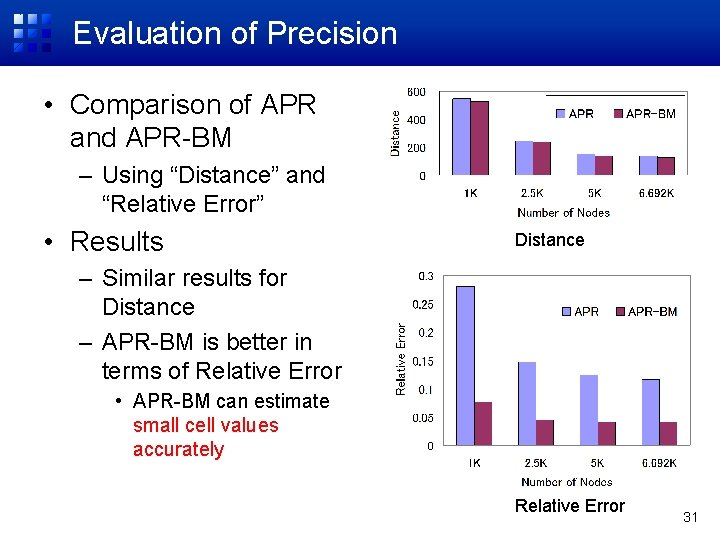
Evaluation of Precision • Comparison of APR and APR-BM – Using “Distance” and “Relative Error” • Results Distance – Similar results for Distance – APR-BM is better in terms of Relative Error • APR-BM can estimate small cell values accurately Relative Error 31
Outline • • • Background and Objectives Modeling Movement Patterns Mobility Histogram: Logical Structure Mobility Histogram: Physical Structure Experimental Results Conclusions 32
Conclusions • Mobility histogram construction method – Based on Markov chain model – Handling streamed trajectory sequences – Logical histogram: data cube – Physical histogram: tree structure (quad tree + k-d tree) • Adaptive tree growth • Approximated representation method • Use of nonparametric statistics for exceptional cases • Use of a bitmap cube to enhance precision 33
- Slides: 34