A Computational Study of Three Demon Algorithm Variants

A Computational Study of Three Demon Algorithm Variants for Solving the TSP by Bala Chandran, University of Maryland Bruce Golden, University of Maryland Edward Wasil, American University Presented at Phoenix ICS Conference, January 2003

Focus of Paper g Review previous work i i i simulated annealing (SA) the demon algorithm preliminary computational work g Introduce three new demon algorithm variants g Perform a computational study g Present conclusions 2

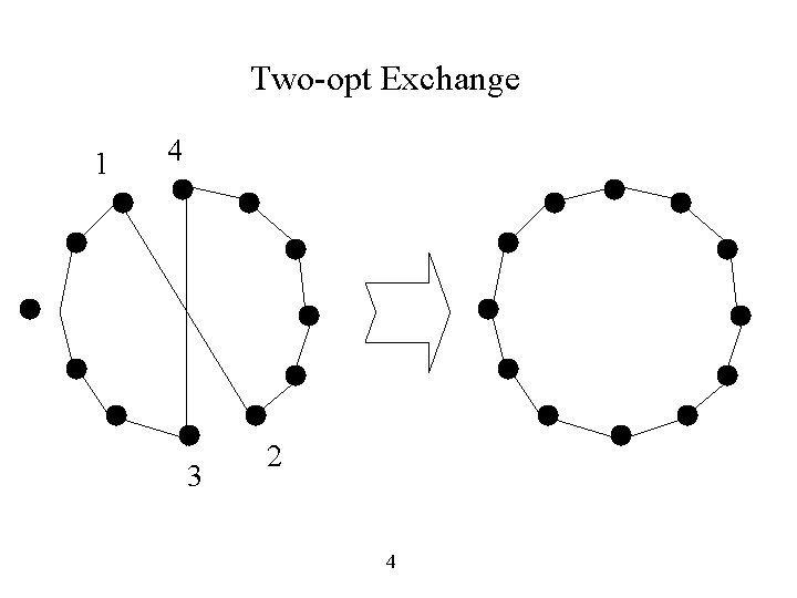
Metaheuristics g Work in this direction began with simulated annealing (1983) g Metaheuristics for the TSP are often based on the concept of arc exchanges (dating back to the two-opt) g The starting point was to realize that occasionally accepting arc exchanges that increased tour length was okay 3

Two-opt Exchange 1 4 3 2 4

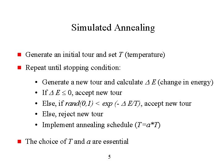
Simulated Annealing g Generate an initial tour and set T (temperature) g Repeat until stopping condition: i i i g Generate a new tour and calculate E (change in energy) If E 0, accept new tour Else, if rand(0, 1) < exp (- E/T), accept new tour Else, reject new tour Implement annealing schedule (T=a*T) The choice of T and a are essential 5

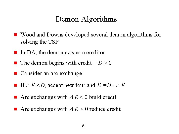
Demon Algorithms g Wood and Downs developed several demon algorithms for solving the TSP g In DA, the demon acts as a creditor g The demon begins with credit = D > 0 g Consider an arc exchange g If E <D, accept new tour and D =D - E g Arc exchanges with E < 0 build credit g Arc exchanges with E > 0 reduce credit 6

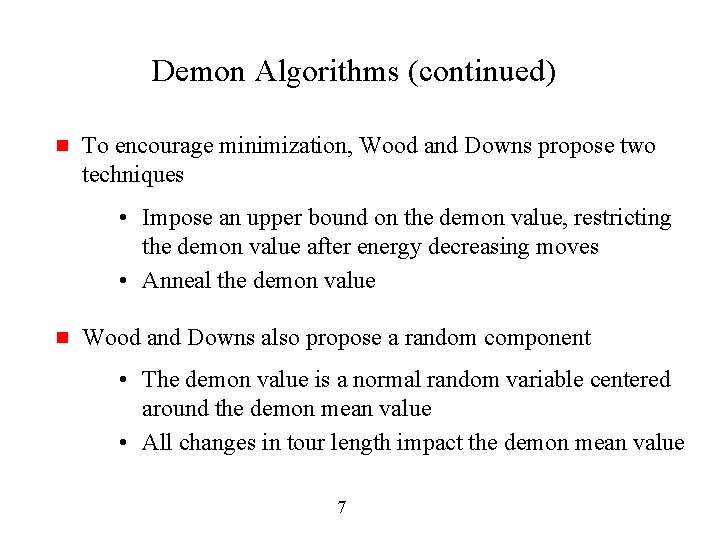
Demon Algorithms (continued) g To encourage minimization, Wood and Downs propose two techniques i i g Impose an upper bound on the demon value, restricting the demon value after energy decreasing moves Anneal the demon value Wood and Downs also propose a random component i i The demon value is a normal random variable centered around the demon mean value All changes in tour length impact the demon mean value 7

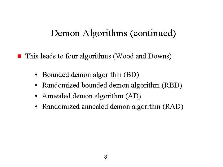
Demon Algorithms (continued) g This leads to four algorithms (Wood and Downs) i i Bounded demon algorithm (BD) Randomized bounded demon algorithm (RBD) Annealed demon algorithm (AD) Randomized annealed demon algorithm (RAD) 8

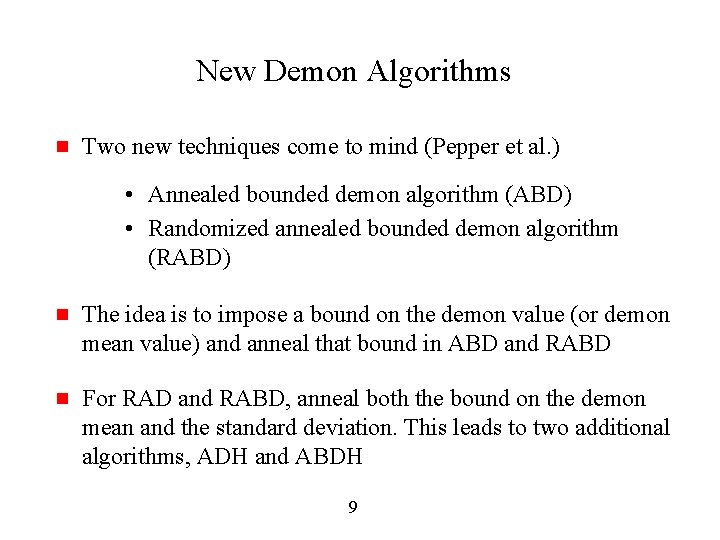
New Demon Algorithms g Two new techniques come to mind (Pepper et al. ) i i Annealed bounded demon algorithm (ABD) Randomized annealed bounded demon algorithm (RABD) g The idea is to impose a bound on the demon value (or demon mean value) and anneal that bound in ABD and RABD g For RAD and RABD, anneal both the bound on the demon mean and the standard deviation. This leads to two additional algorithms, ADH and ABDH 9

Computational Study g Eleven algorithms in all g We selected 29 instances from TSPLIB g The instances range in size from 105 to 1, 432 nodes g The instances have different structures g Each algorithm was applied 25 times to each instance from a randomized greedy start g Best and average performance and running time statistics were gathered 10

Parameter Settings g We selected three representative test instances i g For each algorithm, a GA determines a set of parameter values (parameter vector) that works well on these instances Resulting parameter vector is applied to all 29 instances 11

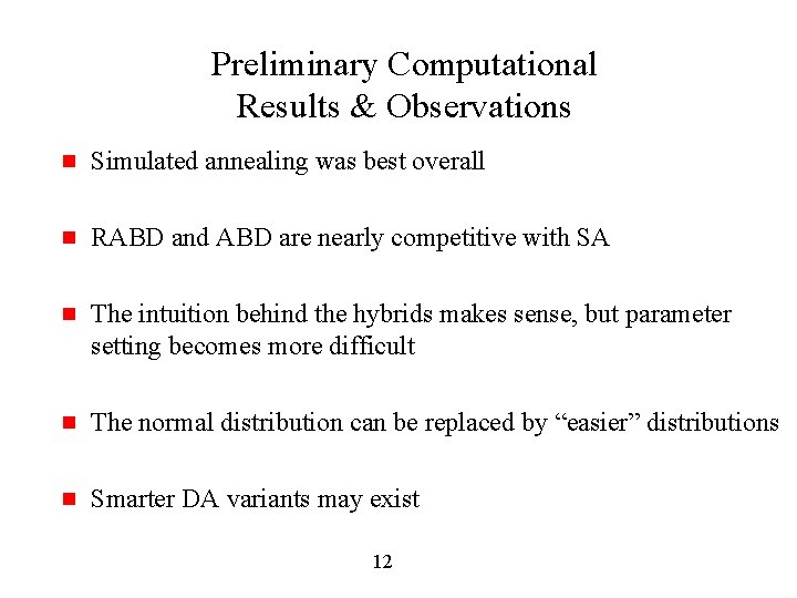
Preliminary Computational Results & Observations g Simulated annealing was best overall g RABD and ABD are nearly competitive with SA g The intuition behind the hybrids makes sense, but parameter setting becomes more difficult g The normal distribution can be replaced by “easier” distributions g Smarter DA variants may exist 12

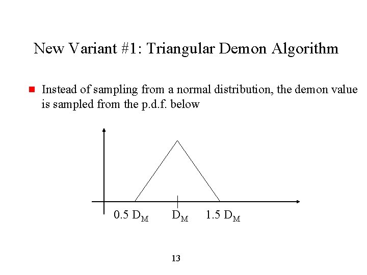
New Variant #1: Triangular Demon Algorithm g Instead of sampling from a normal distribution, the demon value is sampled from the p. d. f. below 0. 5 DM DM 13 1. 5 DM

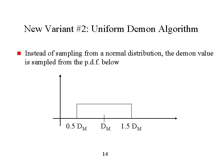
New Variant #2: Uniform Demon Algorithm g Instead of sampling from a normal distribution, the demon value is sampled from the p. d. f. below 0. 5 DM DM 14 1. 5 DM

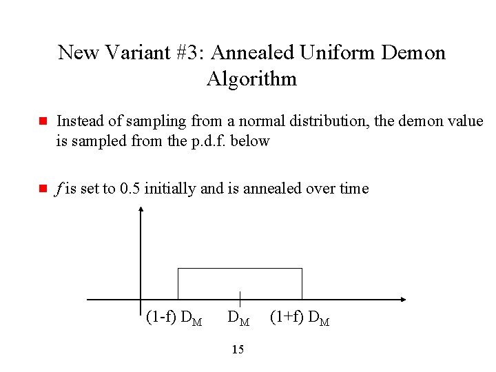
New Variant #3: Annealed Uniform Demon Algorithm g Instead of sampling from a normal distribution, the demon value is sampled from the p. d. f. below g f is set to 0. 5 initially and is annealed over time (1 -f) DM DM 15 (1+f) DM

Advantages of New Variants g Only two parameters need to be set (initial demon value and annealing schedule) – same as for SA g The mean and standard deviation are annealed at the same time g Sampling is easier in these three cases than sampling from a normal distribution 16

Experimental Design g We selected 36 symmetric, Euclidean instances from TSPLIB g The instances range in size from 105 to 1, 432 nodes g For each algorithm, parameters were set using a GA-based procedure on a small subset of the instances 17

Experimental Design (continued) g Starting tour i greedy heuristic i savings heuristic g Tour improvement using 2 -opt g Termination condition: 50 iterations of no improvement after going below the initial tour length or a maximum of 500 iterations 18

Experimental Design (continued) g Each algorithm was run 25 times for each of the 36 instances g Averaged results are presented g All runs were carried out on a Sun Ultra 10 workstation on a Solaris 7 platform g The six best algorithms are compared 19

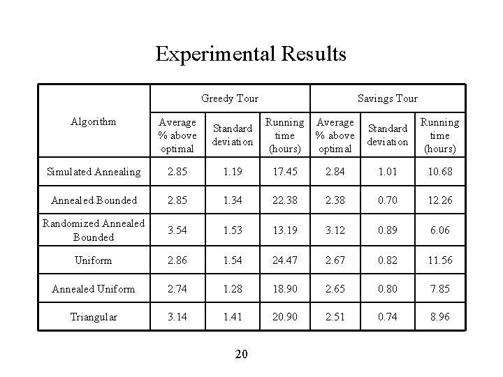
Experimental Results Greedy Tour Savings Tour Algorithm Average % above optimal Standard deviation Running time (hours) Simulated Annealing 2. 85 1. 19 17. 45 2. 84 1. 01 10. 68 Annealed Bounded 2. 85 1. 34 22. 38 0. 70 12. 26 Randomized Annealed Bounded 3. 54 1. 53 13. 19 3. 12 0. 89 6. 06 Uniform 2. 86 1. 54 24. 47 2. 67 0. 82 11. 56 Annealed Uniform 2. 74 1. 28 18. 90 2. 65 0. 80 7. 85 Triangular 3. 14 1. 41 20. 90 2. 51 0. 74 8. 96 20

Conclusions 1. With a greedy start, Annealed Uniform is best 1. When the savings heuristic is used at the start 1. Annealed Bounded is best i Triangular and Annealed Uniform also perform well and beat SA Demon algorithms are sensitive to the starting conditions i 1. Using the savings heuristic significantly reduces computation times Demon algorithms can be applied to other combinatorial optimization problems 21