A Comparison of Lauritzen Spiegelhalter Hugin and Shenoy

A Comparison of Lauritzen. Spiegelhalter, Hugin, and Shenoy -Shafer Architectures for Computing Marginals of Probability Distributions Scott Langevin Chris Streett Alicia Ruvinsky UNIVERSITY OF SOUTH CAROLINA Department of Computer Science and Engineering

History • Computing Marginals of Multivariate Discrete probability distributions in Uncertain reasoning • 1986 – Pearl’s architecture – Singly connected Bayes nets – Singly connected = (a. k. a. polytree) there exists at most one path between any 2 nodes • 1988 – Lauritzen and Spiegelhalter create LS • 1990 – Jensen et al. modify LS creating Hugin • 1990 – Inspired by previous work, Shenoy and Shafer propose framework using join trees to produce marginals • 1997 – Shenoy refines Shenoy-Shafer architecture with binary join trees – This will be referred to as the Shenoy-Shafer (SS) architecture UNIVERSITY OF SOUTH CAROLINA Department of Computer Science and Engineering

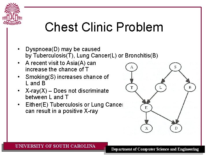
Chest Clinic Problem • Dyspnoea(D) may be caused by Tuberculosis(T), Lung Cancer(L) or Bronchitis(B) • A recent visit to Asia(A) can increase the chance of T • Smoking(S) increases chance of L and B • X-ray(X) – Does not discriminate between L and T • Either(E) Tuberculosis or Lung Cancer can result in a positive X-ray UNIVERSITY OF SOUTH CAROLINA Department of Computer Science and Engineering

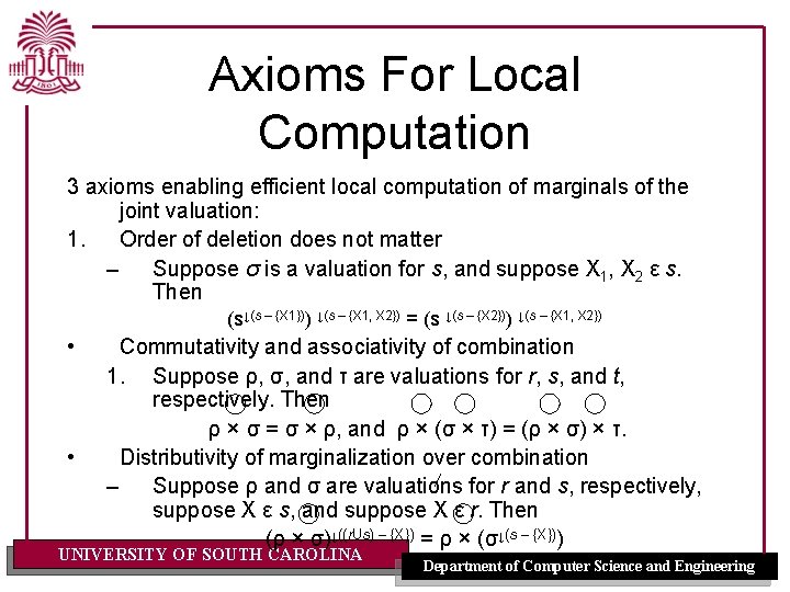
Axioms For Local Computation 3 axioms enabling efficient local computation of marginals of the joint valuation: 1. Order of deletion does not matter – Suppose σ is a valuation for s, and suppose X 1, X 2 ε s. Then (s↓(s – {X 1})) ↓(s – {X 1, X 2}) = (s ↓(s – {X 2})) ↓(s – {X 1, X 2}) • • Commutativity and associativity of combination 1. Suppose ρ, σ, and τ are valuations for r, s, and t, respectively. Then ρ × σ = σ × ρ, and ρ × (σ × τ) = (ρ × σ) × τ. Distributivity of marginalization over combination – Suppose ρ and σ are valuations for r and s, respectively, suppose X ε s, and suppose X ε r. Then (ρ × σ)↓((r. Us) – {X}) = ρ × (σ↓(s – {X})) UNIVERSITY OF SOUTH CAROLINA Department of Computer Science and Engineering

Lauritzen-Spiegelhalter Architecture – Junction Trees • First construct junction tree for BN – Join tree where each node is a clique • Associate each potential Kv with smallest clique that contains {V} U Pa(V). If clique contains more than one potential associate cartesian product of potentials to clique • Evidence is modeled as potentials and associated with smallest clique that includes domain of potential • Pick a node with largest state space in junction tree to be root UNIVERSITY OF SOUTH CAROLINA Department of Computer Science and Engineering

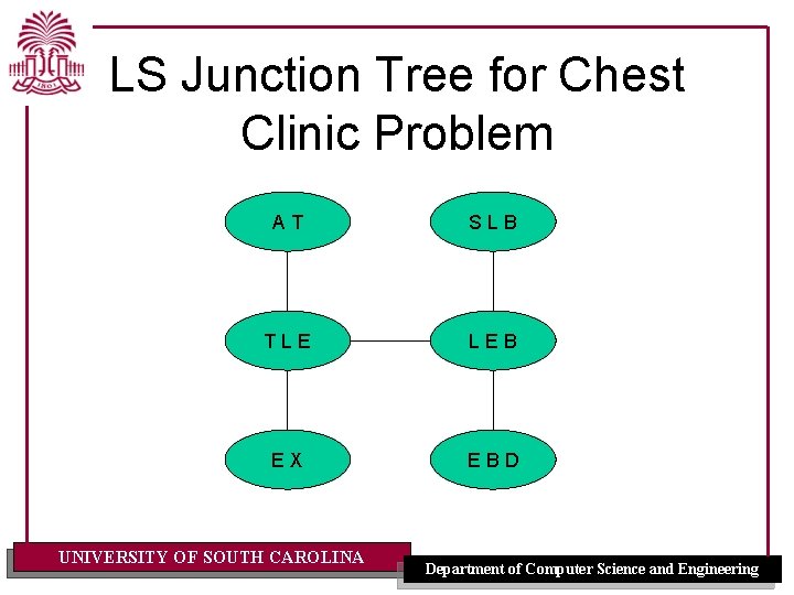
LS Junction Tree for Chest Clinic Problem AT SLB TLE LEB EX EBD UNIVERSITY OF SOUTH CAROLINA Department of Computer Science and Engineering

• • • Lauritzen-Spiegelhalter Architecture - Calculating Marginals Two phases: Inward pass, Outward pass Involves sending messages which are potentials to neighboring nodes Inward pass – Each node sends message to inward neighbor after it receives messages from all outward neighbors. If no outward neighbors, send message. – When sending, message is computed by marginalizing current potential to intersection with inward neighbor. Message is sent to inward neighbor and current potential is divided by message – When receiving message from outward neighbor, current potential is multiplied by message – Inward pass ends when root has received a message from all outward neighbors UNIVERSITY OF SOUTH CAROLINA Department of Computer Science and Engineering

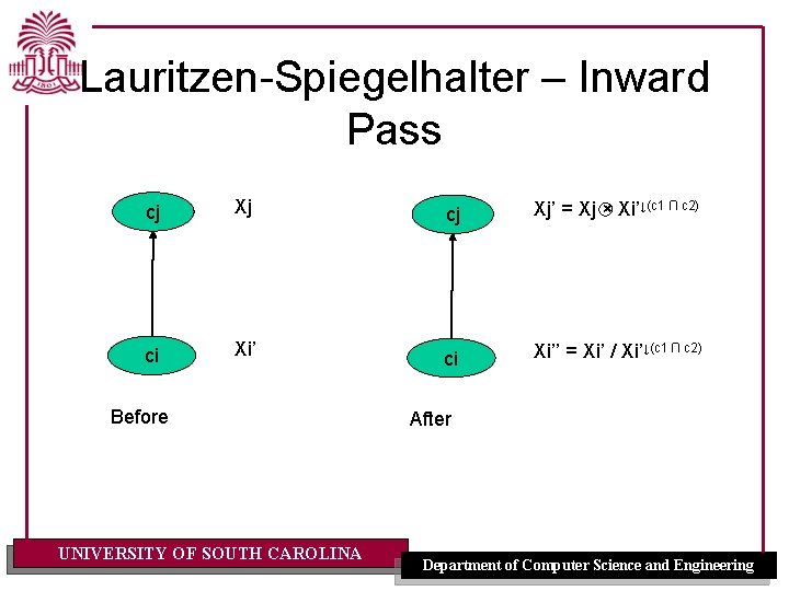
Lauritzen-Spiegelhalter – Inward Pass cj Xj’ = Xj × Xi’↓(c 1 ∩ c 2) ci Xi’’ = Xi’ / Xi’↓(c 1 ∩ c 2) Before UNIVERSITY OF SOUTH CAROLINA After Department of Computer Science and Engineering

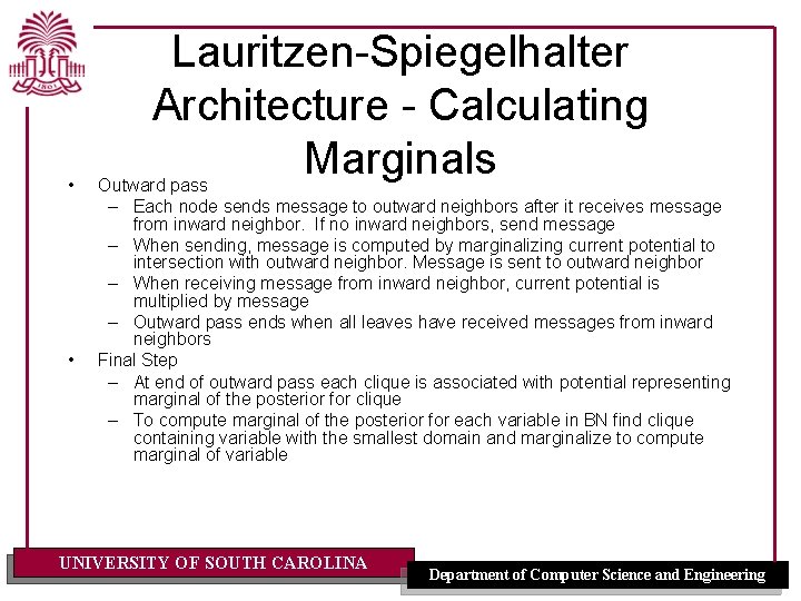
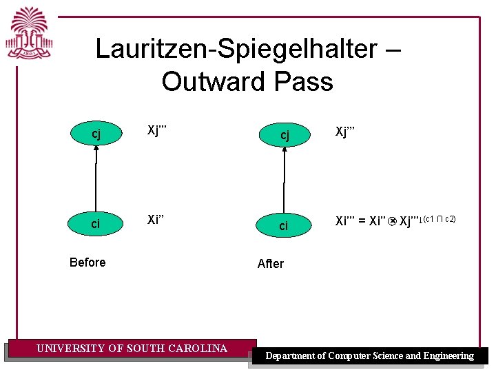
• • Lauritzen-Spiegelhalter Architecture - Calculating Marginals Outward pass – Each node sends message to outward neighbors after it receives message from inward neighbor. If no inward neighbors, send message – When sending, message is computed by marginalizing current potential to intersection with outward neighbor. Message is sent to outward neighbor – When receiving message from inward neighbor, current potential is multiplied by message – Outward pass ends when all leaves have received messages from inward neighbors Final Step – At end of outward pass each clique is associated with potential representing marginal of the posterior for clique – To compute marginal of the posterior for each variable in BN find clique containing variable with the smallest domain and marginalize to compute marginal of variable UNIVERSITY OF SOUTH CAROLINA Department of Computer Science and Engineering

Lauritzen-Spiegelhalter – Outward Pass cj Xj’’’ ci Xi’’’ = Xi’’ × Xj’’’↓(c 1 ∩ c 2) Before UNIVERSITY OF SOUTH CAROLINA After Department of Computer Science and Engineering

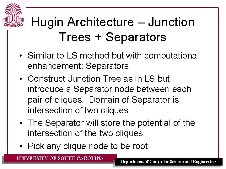
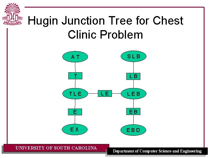
Hugin Architecture – Junction Trees + Separators • Similar to LS method but with computational enhancement: Separators • Construct Junction Tree as in LS but introduce a Separator node between each pair of cliques. Domain of Separator is intersection of two cliques. • The Separator will store the potential of the intersection of the two cliques • Pick any clique node to be root UNIVERSITY OF SOUTH CAROLINA Department of Computer Science and Engineering

Hugin Junction Tree for Chest Clinic Problem AT SLB TLE LE LEB EX EBD UNIVERSITY OF SOUTH CAROLINA Department of Computer Science and Engineering

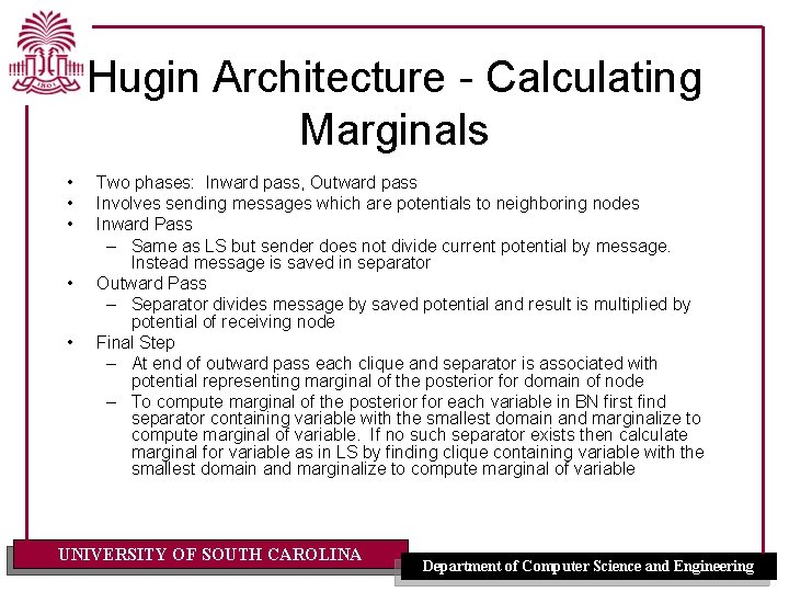
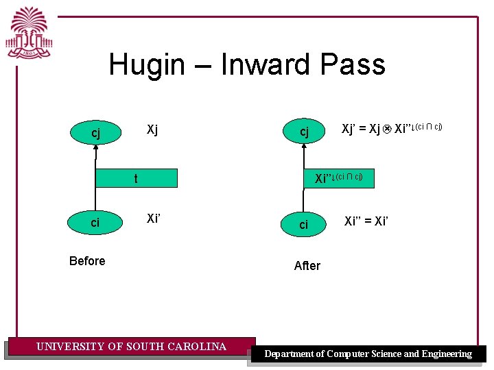
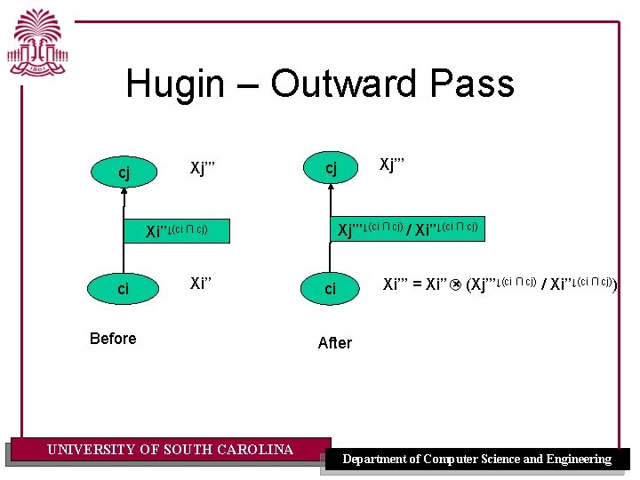
Hugin Architecture - Calculating Marginals • • • Two phases: Inward pass, Outward pass Involves sending messages which are potentials to neighboring nodes Inward Pass – Same as LS but sender does not divide current potential by message. Instead message is saved in separator Outward Pass – Separator divides message by saved potential and result is multiplied by potential of receiving node Final Step – At end of outward pass each clique and separator is associated with potential representing marginal of the posterior for domain of node – To compute marginal of the posterior for each variable in BN first find separator containing variable with the smallest domain and marginalize to compute marginal of variable. If no such separator exists then calculate marginal for variable as in LS by finding clique containing variable with the smallest domain and marginalize to compute marginal of variable UNIVERSITY OF SOUTH CAROLINA Department of Computer Science and Engineering

Hugin – Inward Pass Xj cj t ci Xj’ = Xj × Xi’’↓(ci ∩ cj) cj Xi’’↓(ci ∩ cj) Xi’ Before UNIVERSITY OF SOUTH CAROLINA ci Xi’’ = Xi’ After Department of Computer Science and Engineering

Hugin – Outward Pass cj Xj’’’↓(ci ∩ cj) / Xi’’↓(ci ∩ cj) ci Xi’’ Before UNIVERSITY OF SOUTH CAROLINA Xj’’’ cj Xi’’’ = Xi’’ × (Xj’’’↓(ci ∩ cj) / Xi’’↓(ci ∩ cj)) ci After Department of Computer Science and Engineering

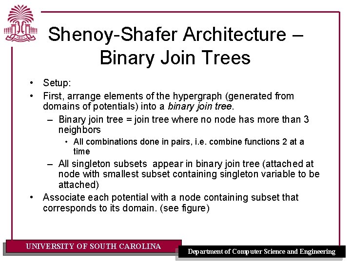
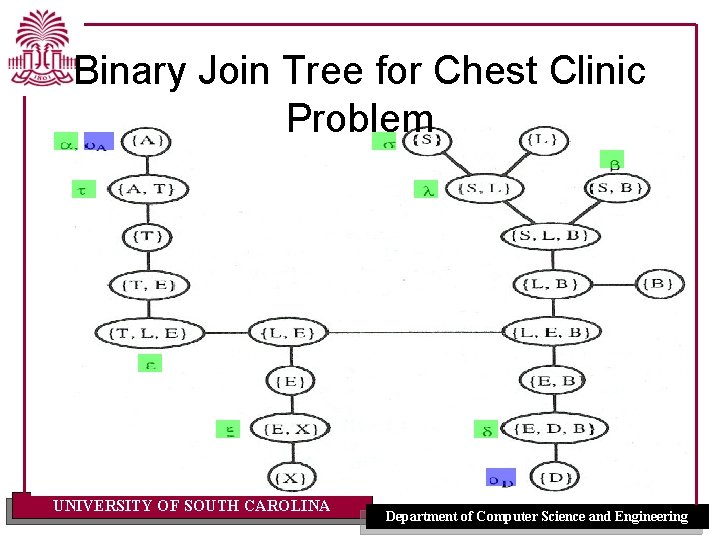
Shenoy-Shafer Architecture – Binary Join Trees • Setup: • First, arrange elements of the hypergraph (generated from domains of potentials) into a binary join tree. – Binary join tree = join tree where no node has more than 3 neighbors • All combinations done in pairs, i. e. combine functions 2 at a time – All singleton subsets appear in binary join tree (attached at node with smallest subset containing singleton variable to be attached) • Associate each potential with a node containing subset that corresponds to its domain. (see figure) UNIVERSITY OF SOUTH CAROLINA Department of Computer Science and Engineering

Binary Join Tree for Chest Clinic Problem UNIVERSITY OF SOUTH CAROLINA Department of Computer Science and Engineering

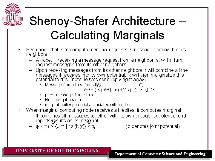
Shenoy-Shafer Architecture – Calculating Marginals • • Each node that is to compute marginal requests a message from each of its neighbors – A node, r, receiving a message request from a neighbor, s, will in turn request messages from its other neighbors – Upon receiving messages from its other neighbors, r will combine all the messages it receives into its own potential. R will then marginalize this potential to r∩s. (note: leaves send reply right away) • Message from r to s, formally: μr→s = ( × {μt→r | t ε (N(r) {s}) } × αr}↓r∩s • μr→s : message from r to s • N(r) : neighbors of r • αr : probability potential associated with node r When marginal computing node receives all replies, it computes marginal – It combines all messages together with its own probability potential and reports results as its marginal. – φ ↓r = ( × {μt→r | t ε (N(r)} × αr (φ denotes joint potential) UNIVERSITY OF SOUTH CAROLINA Department of Computer Science and Engineering

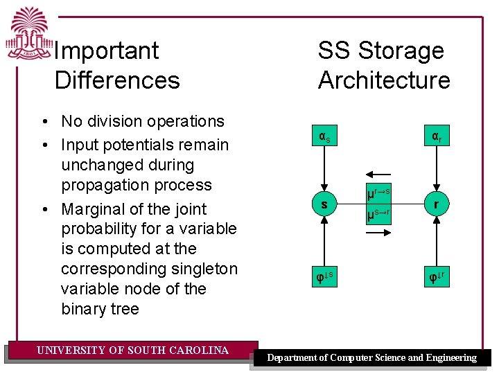
Important Differences • No division operations • Input potentials remain unchanged during propagation process • Marginal of the joint probability for a variable is computed at the corresponding singleton variable node of the binary tree UNIVERSITY OF SOUTH CAROLINA SS Storage Architecture αs s φ↓s αr μr→s μs→r r φ↓r Department of Computer Science and Engineering

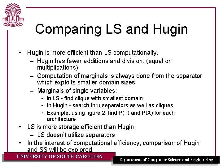
Comparing LS and Hugin • Hugin is more efficient than LS computationally. – Hugin has fewer additions and division. (equal on multiplications) – Computation of marginals is always done from the separator which exploits smaller domain sizes. – Marginals of single variables: • in LS - find clique with smallest domain • In Hugin - search thru separators as well as cliques • Example: using figure 2, find P(T) and P(X) for each architecture • LS is more storage efficient than Hugin. – LS doesn’t utilize separators • In the interest of computational efficiency, comparison of Hugin and SS will be explored. UNIVERSITY OF SOUTH CAROLINA Department of Computer Science and Engineering

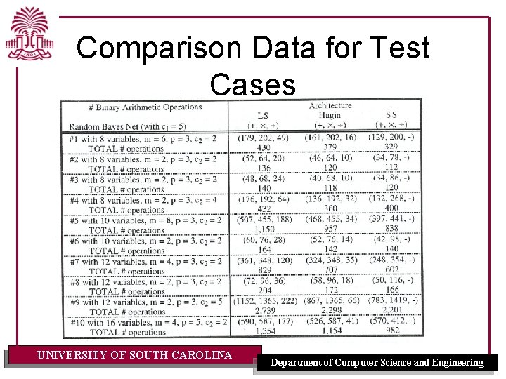
Comparing Hugin and SS • SS is more computationally efficient than Hugin – SS has no divisions (on average, less computations) – Efficiency of SS increases with larger state spaces – Calculating probability of singleton variables • adds expense in Hugin • always calculated and available in SS. • SS is more flexible than Hugin (as well as LS) – Due to lack of division • CONJECTURE: Hugin is more storage efficient than SS. – To be investigated – SS has a larger data structure, hence most likely uses more space UNIVERSITY OF SOUTH CAROLINA Department of Computer Science and Engineering

Comparison Data for Test Cases UNIVERSITY OF SOUTH CAROLINA Department of Computer Science and Engineering