A case example Building a population pharmacokinetic model

A case example: Building a population pharmacokinetic model for theophylline using NONMEM program. Pyry Välitalo Orion Pharma Orion Corporation Pyry Välitalo SSL Presentation 2. 2. 2010 1

Population pharmacokinetics: Pharmacokinetics using nonlinear mixed-effects models • Rather than model each individuals’ response separately, combine all the data in one model. The differences between individuals are described with random effects. • Benefit: Possible to use data that would not be adequate for individual PK modeling (e. g. sparse sampling). • Benefit: More data per model yields more power. – One model for each individual versus one model for all data • Benefit: Easier to ”locate” sources of between-subject variability? Orion Corporation Pyry Välitalo SSL Presentation 1. 1. 2007 2

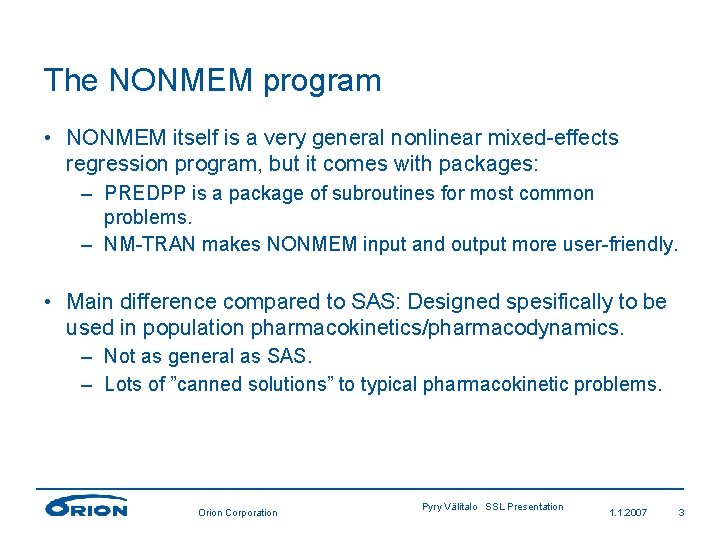
The NONMEM program • NONMEM itself is a very general nonlinear mixed-effects regression program, but it comes with packages: – PREDPP is a package of subroutines for most common problems. – NM-TRAN makes NONMEM input and output more user-friendly. • Main difference compared to SAS: Designed spesifically to be used in population pharmacokinetics/pharmacodynamics. – Not as general as SAS. – Lots of ”canned solutions” to typical pharmacokinetic problems. Orion Corporation Pyry Välitalo SSL Presentation 1. 1. 2007 3

Some nomenclature • Fixed effects: Theta, θ. Mostly used to describe the structural model (e. g. clearance) and covariate relationships (e. g. effect of sex on clearance) – In general statistical nomenclature: b • Random effects: Eta, η. The standard deviation of the random effects is ω. In population pharmacokinetics, random effects are most commonly used to describe between-subject variability. – In general statistical nomenclature: bi • Residual variability: Epsilon, ε. The standard deviation of the residual variability is σ. – The general statistical nomenclature is similar? Orion Corporation Pyry Välitalo SSL Presentation 2. 2. 2010 4

The dataset (theophylline): • Part of the data used in: Upton RA, Thiercelin JF, Guentert TW, Wallace SM, Powell JR, Sansom L, Riegelman S. Intraindividual variability in theophylline pharmacokinetics: statistical verification in 39 of 60 healthy young adults. J Pharmacokinet Biopharm. 1982 Apr; 10(2): 12334. • The dataset comes with NONMEM software. Orion Corporation Pyry Välitalo SSL Presentation 2. 2. 2010 5

The dataset • 12 individuals given a single dose of 3 -6 mg/kg of oral theophylline. • 10 concentration measurements from 25 hours – A total of 120 observations • One continuous covariate: Weight. Orion Corporation Pyry Välitalo SSL Presentation 2. 2. 2010 6

ADVAN 2 subroutine: The subroutine to be used throughout this example. • ADVAN 2 subroutine is used throughout the example. This subroutine defines an absorption compartment and a central compartment. • ADVAN 2 requires the following to be specified: – KA (absorption rate constant) – K (elimination rate constant) – How the observations are scaled (i. e. how do the drug amounts relate to concentrations)? – How the observation and individual prediction relate to each other, i. e. what type of residual error is used? – Everything else is optional. Orion Corporation Pyry Välitalo SSL Presentation 1. 1. 2007 7

Oral pharmacokinetic data and ADVAN 2 subroutine • In its most basic form: At t=0 A(1)=Dose and A(2)=0 d. A(1)/dt=-KA*A(1) d. A(2)/dt=KA*A(1)-K*A(2) Depot(1) KA Central(2) K • Define e. g. that – – KA=THETA(1) * EXP(ETA(1)) K=THETA(2) * EXP(ETA(2)) V=THETA(3) * EXP(ETA(3)) ; Volume of distribution Y=A(2)/V + EPS(1) ; observation is the predicted ; concentration plus residual error Orion Corporation Pyry Välitalo SSL Presentation 1. 1. 2007 8

Run 1: ”The zero model” • This control stream came with the dataset, and likely originates from year 1982: $SUBROUTINES ADVAN 2 KA=THETA(1)+ETA(1) K=THETA(2)+ETA(2) CL=THETA(3)*WT+ETA(3) SC=CL/K/WT ; absorption rate constant ; elimination rate constant ; clearance is scaled by weight ; scaling of concentration observations is done ; by calculating V=CL/K and scaling by weight ; because dose is weight-adjusted. $THETA (. 1, 3, 5) (. 008, . 5) (. 004, . 9) ; Fixed effects estimates $OMEGA BLOCK(3) 6. 005. 0002. 3. 006. 4 ; Random effects variance-covariance $ERROR Y=F+EPS(1) ; additive error model $SIGMA ; Residual error variance estimate $EST . 4 MAXEVAL=450 PRINT=5 ; First Order method Orion Corporation Pyry Välitalo SSL Presentation 2. 2. 2010 9

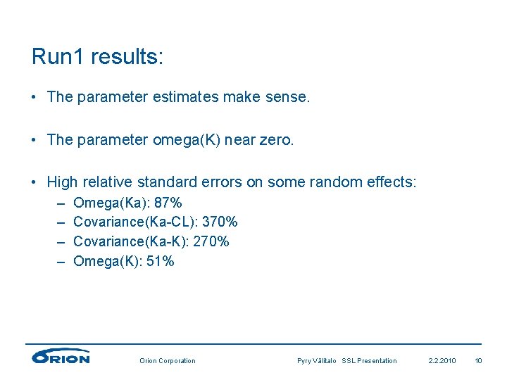
Run 1 results: • The parameter estimates make sense. • The parameter omega(K) near zero. • High relative standard errors on some random effects: – – Omega(Ka): 87% Covariance(Ka-CL): 370% Covariance(Ka-K): 270% Omega(K): 51% Orion Corporation Pyry Välitalo SSL Presentation 2. 2. 2010 10

Run 1 results: Plasma concentrations and predictions. Orion Corporation Pyry Välitalo SSL Presentation 2. 2. 2010 11

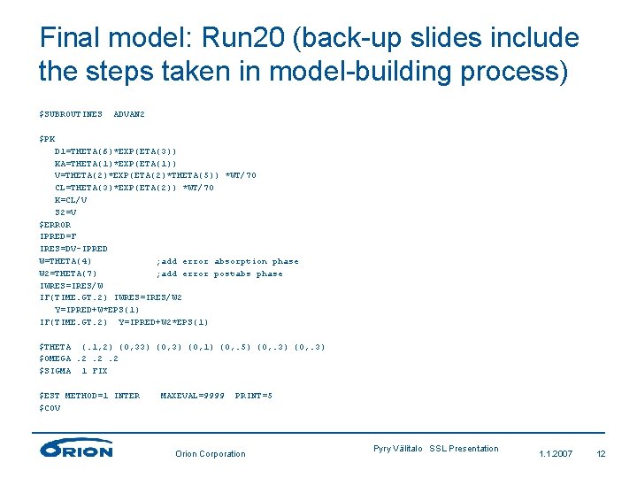
Final model: Run 20 (back-up slides include the steps taken in model-building process) $SUBROUTINES ADVAN 2 $PK D 1=THETA(6)*EXP(ETA(3)) KA=THETA(1)*EXP(ETA(1)) V=THETA(2)*EXP(ETA(2)*THETA(5)) *WT/70 CL=THETA(3)*EXP(ETA(2)) *WT/70 K=CL/V S 2=V $ERROR IPRED=F IRES=DV-IPRED W=THETA(4) ; add error absorption phase W 2=THETA(7) ; add error postabs phase IWRES=IRES/W IF(TIME. GT. 2) IWRES=IRES/W 2 Y=IPRED+W*EPS(1) IF(TIME. GT. 2) Y=IPRED+W 2*EPS(1) $THETA (. 1, 2) (0, 33) (0, 1) (0, . 5) (0, . 3) $OMEGA. 2. 2. 2 $SIGMA 1 FIX $EST METHOD=1 INTER $COV MAXEVAL=9999 PRINT=5 Orion Corporation Pyry Välitalo SSL Presentation 1. 1. 2007 12

Aspects of the improved model: Residual error model $SUBROUTINES ADVAN 2 $PK D 1=THETA(6)*EXP(ETA(3)) KA=THETA(1)*EXP(ETA(1)) V=THETA(2)*EXP(ETA(2)*THETA(5)) *WT/70 CL=THETA(3)*EXP(ETA(2)) *WT/70 K=CL/V S 2=V $ERROR IPRED=F IRES=DV-IPRED W=THETA(4) ; additive error defined with fixed effect. THETA(4) equals sd of res. var. W 2=THETA(7) ; additive error defined with fixed effect. THETA(7) equals sd of res. var. IWRES=IRES/W ; IWRES are weighted with standard deviation of residual variability IF(TIME. GT. 2) IWRES=IRES/W 2 ; for post-absorption period Y=IPRED+W*EPS(1) ; multiply by W because sd of residual variability is fixed to 1. IF(TIME. GT. 2) Y=IPRED+W 2*EPS(1) ; for post-absorption period $THETA (. 1, 2) (0, 33) (0, 1) (0, . 5) (0, . 3) $OMEGA. 2. 2. 2 $SIGMA 1 FIX ; Variance of EPS(1) values is fixed to 1. $EST METHOD=1 INTER $COV MAXEVAL=9999 PRINT=5 Orion Corporation Pyry Välitalo SSL Presentation 1. 1. 2007 13

Benefits of coding residual error model this way: • We can obtain IWRES values as per definition: IWRES = (observation – IPRED)/σ (e. g. Karlsson & Savic 2005) – This is used to standardize the IWRES, so that they should have a standard deviation of 1 (and mean of 0). • Sometimes, using a fixed effect makes the model more stable than estimating a lot of random effects. • Regarding the use of separate residual errors for absorption and post-absorption phases: This makes sense because the absorption phase typically has more ”noise” than postabsorption phase (and IV data is yet more reliable). – Has been proposed in some articles, e. g. Karlsson MO, Beal SL, Sheiner LB. J Pharmacokinet Biopharm. 1995 Dec; 23(6): 651 -72. Chan PL, Weatherley B, Mc. Fadyen L. Br J Clin Pharmacol. 2008 Apr; 65 Suppl 1: 76 -85. Orion Corporation Pyry Välitalo SSL Presentation 1. 1. 2007 14

Aspects of the improved model: Distribution of random effects, estimation method, implementing weight as a covariate $SUBROUTINES ADVAN 2 ; This is a predefined subroutine for 1 -compartment model ; with first order absorption $PK D 1=THETA(6)*EXP(ETA(3)) KA=THETA(1)*EXP(ETA(1)) V=THETA(2)*EXP(ETA(2)*THETA(5)) *WT/70 CL=THETA(3)*EXP(ETA(2)) *WT/70 K=CL/V S 2=V $ERROR IPRED=F IRES=DV-IPRED W=THETA(4) ; add error W 2=THETA(7) ; add err postabs IWRES=IRES/W IF(TIME. GT. 2) IWRES=IRES/W 2 Y=IPRED+W*EPS(1) IF(TIME. GT. 2) Y=IPRED+W 2*EPS(1) ; log-normal distribution, linear scaling by weight $THETA (. 1, 2) (0, 33) (0, 1) (0, . 5) (0, . 3) $OMEGA. 2. 2. 2 $SIGMA 1 FIX $EST METHOD=1 INTER $COV MAXEVAL=9999 PRINT=5 Orion Corporation ; method is First Order Conditional Estimation with ; Interaction Pyry Välitalo SSL Presentation 1. 1. 2007 15

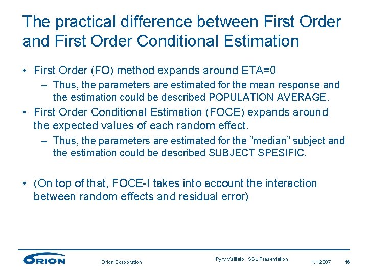
The practical difference between First Order and First Order Conditional Estimation • First Order (FO) method expands around ETA=0 – Thus, the parameters are estimated for the mean response and the estimation could be described POPULATION AVERAGE. • First Order Conditional Estimation (FOCE) expands around the expected values of each random effect. – Thus, the parameters are estimated for the ”median” subject and the estimation could be described SUBJECT SPESIFIC. • (On top of that, FOCE-I takes into account the interaction between random effects and residual error) Orion Corporation Pyry Välitalo SSL Presentation 1. 1. 2007 16

Implementing bodyweight in the model • Linear scaling of both clearance and volume of distribution by bodyweight. • Current trend, at least for pediatrics: linear scaling for volume of distribution, nonlinear scaling for clearance (estimate an exponent for nonlinear scaling). – Probably not applicable to obese patients, etc. • Weight range in this data 55 -86 kg (median 70 kg). – Probably not wide enough range to estimate nonlinearity. Orion Corporation Pyry Välitalo SSL Presentation 1. 1. 2007 17

Aspects of the improved model: Absorption model $SUBROUTINES ADVAN 2 $PK D 1=THETA(6)*EXP(ETA(3)) ; D 1=duration of a hypothetical infusion into the depot ; compartment KA=THETA(1)*EXP(ETA(1)) V=THETA(2)*EXP(ETA(2)*THETA(5)) *WT/70 CL=THETA(3)*EXP(ETA(2)) *WT/70 K=CL/V S 2=V $ERROR IPRED=F IRES=DV-IPRED W=THETA(4) ; add error W 2=THETA(7) ; add err postabs IWRES=IRES/W IF(TIME. GT. 2) IWRES=IRES/W 2 Y=IPRED+W*EPS(1) IF(TIME. GT. 2) Y=IPRED+W 2*EPS(1) $THETA (. 1, 2) (0, 33) (0, 1) (0, . 5) (0, . 3) $OMEGA. 2. 2. 2 $SIGMA 1 FIX $EST METHOD=1 INTER $COV MAXEVAL=9999 PRINT=5 Orion Corporation Pyry Välitalo SSL Presentation 1. 1. 2007 18

The absorption model: Mixed 0 - and 1 storder absorption. If (time<D 1) d. A(1)/dt=Dose/D 1 –KA*A(1) If (time>D 1) d. A(1)/dt=–KA*A(1) • A lagtime model was also tried but the mixed 0 - and 1 st-order absorption proved better with the following benefits: – Describes the data better (lower OFV) – Would make it possible to use proportional error model? – Not as ”radical” a change point as lagtime: possibly more stable than using lagtime? • Probably better still: Transit compartmental absorption (was not tried in this case because of time limitations). – Savic RM, Jonker DM, Kerbusch T, Karlsson MO. J Pharmacokinet Pharmacodyn. 2007 Oct; 34(5): 711 -26. Epub 2007 Jul 26. Orion Corporation Pyry Välitalo SSL Presentation 1. 1. 2007 19

What was the additional effort worth? • Compared to the original run we have: – More complicated absorption model. – More complicated residual error model. – (No random effect for elimination rate constant). • What did we benefit from this? – A better absorption model may also result in more accurate estimates of V/F and CL/F. – Since different magnitudes of residual error are identified for absorption and post-absorption phases, the model has better simulation properties. – The model overall describes the data better (lower residual error). Orion Corporation Pyry Välitalo SSL Presentation 2. 2. 2010 20

Original model parameter estimates versus final model parameter estimates: Parameter Run 3 Run 20 OFV 111 (6 parameters) 1. 84 (10 parameters) KA (1/h) 1. 6 (0. 20) 2. 8 (0. 26) V=CL/K (l) 32 (0. 045) 34 (0. 038) CL (l/h) 2. 7 (0. 079) 2. 7 (0. 074) Omega(KA) 0. 65 (0. 53) 0. 90 (0. 44) Omega(CL) 0. 17 (0. 30) 0. 27 (0. 56) Sigma (mg/l) 0. 71 (0. 13) 0. 66 (0. 15) / 0. 30 (0. 11) *the numbers in parenthesis are relative standard errors Orion Corporation Pyry Välitalo SSL Presentation 2. 2. 2010 21

Take-home messages • If you have problems making the model converge: – Realize that non-continuous functions may be hard to integrate (e. g. lagtime for absorption) – Use the appropriate residual error model. – (In NONMEM: start with a simple model and build ”from ground up”) Orion Corporation Pyry Välitalo SSL Presentation 1. 1. 2007 22

Resources • • • NONMEM. Currently the ”golden standard” in population pharmacokinetic modeling. Requires license. – http: //www. icondevsolutions. com/nonmem. htm Xpose: An R package that helps in deciphering the output of NONMEM. Free. – http: //xpose. sourceforge. net/ R: A program needed by Xpose to operate. Free. – http: //www. r-project. org/ Census. A helpful program for keeping record of NONMEM runs. Free. – http: //census. sourceforge. net/ Ps. N (Perl-speaks-Nonmem). A collection of helpful Perl scripts for NONMEM that make life easier in a lot of ways. Free. MONOLIX. Another population pharmacokinetic program. Free. – Advantages: Shorter runtimes than in NONMEM, provides graphical output by itself. – Disadvantages: Currently not as flexible as NONMEM. May be hard to make sense of the error messages encountered. – http: //software. monolix. org/sdoms/software/ Orion Corporation Pyry Välitalo SSL Presentation 1. 1. 2007 23

(Back-up slides) Run 2: ”Modernize” the original run • Dataset modifications: Input the exact dose that was given to each patient rather than a weight-scaled dose. Input weight as a covariate for every observation. • Rather than model additive random effects, model exponential random effects: THETA(1)+ETA(1) becomes THETA(1)*EXP(ETA(1)) – Because log-normal distributions very typical in pharmacokinetics Orion Corporation Pyry Välitalo SSL Presentation 2. 2. 2010 24

(Back-up slides) Run 2: ”Modernize” the original run • Take away covariance matrix for now, but leave all the random effects parameters. – In NONMEM, unnecessary covariance structures can slow down the estimation and add to model instability. • Instead of First Order (FO) estimation method, use First Order Conditional Estimation with Interaction (FOCE-I) method: In $ESTIMATION block, ”METHOD=1 INTER” line is added – First Order method would expand around ETA=0 (Fixed effects estimated to describe Population Average) – First Order Conditional Estimation with Interaction expands around η=E(η). Thus, the fixed effects describe a typical subject rather than population average (Subject Spesific approximation). Orion Corporation Pyry Välitalo SSL Presentation 1. 1. 2007 25

(Back-up slides) Run 2 results: • OFV 111. 985 • Parameter estimate is near its lower boundary: omega(K) • Left: individual time-concentration plots. Right: Individual random effects KA versus CL. No linear correlation seems to be present; thus, KACL covariance is not implemented. Orion Corporation Pyry Välitalo SSL Presentation 2. 2. 2010 26

(Back-up slides) Forward some runs: • Run 3: Remove random effect on K – OFV 111. 983, large standard error found for omega(KA) • Run 4: Based on run 3. Remove random effect on KA – OFV 186. 687. Even though there is difficulty estimating the random effect, it seems to be an important part of the model. • Run 5: Based on run 3. Implement additive+proportional error. – OFV 105. 320 , large standard error found for omega(KA) • Run 6: Based on run 3. Implement proportional residual error. – OFV 140. 536, fairly large standard error found for omega(KA) • SUMMARY of this slide: The random effect of K (the elimination rate) is not essential to the model. The additive+proportional residual error might improve the model a bit. However, more efforts will be spent on the residual error model later on; that’s why additive+proportional residual error is discontinued. Orion Corporation Author/Department 2. 2. 2010 27

(Back-up slides) Run 7: Based on run 3. Estimate KA, V and CL instead of KA, K and CL: • BEFORE (run 3): KA=THETA(1)*EXP(ETA(1)) K=THETA(2) CL=THETA(3)*EXP(ETA(2)) V=CL/K • AFTER MODIFICATION (run 7): KA=THETA(1)*EXP(ETA(1)) V=THETA(2)*EXP(ETA(2)) CL=THETA(3)*EXP(ETA(2)) K=CL/V • In run 3, it was found that a random effect is not needed for K. Since K=CL/V, in run 7 the same random effect is included for both V and CL. Results identical to run 3 (OFV 111. 983) Orion Corporation Author/Department 2. 2. 2010 28

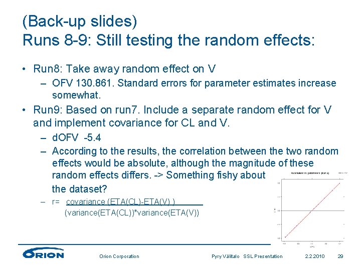
(Back-up slides) Runs 8 -9: Still testing the random effects: • Run 8: Take away random effect on V – OFV 130. 861. Standard errors for parameter estimates increase somewhat. • Run 9: Based on run 7. Include a separate random effect for V and implement covariance for CL and V. – d. OFV -5. 4 – According to the results, the correlation between the two random effects would be absolute, although the magnitude of these random effects differs. -> Something fishy about the dataset? – r= covariance (ETA(CL)-ETA(V) ) (variance(ETA(CL))*variance(ETA(V)) Orion Corporation Pyry Välitalo SSL Presentation 2. 2. 2010 29

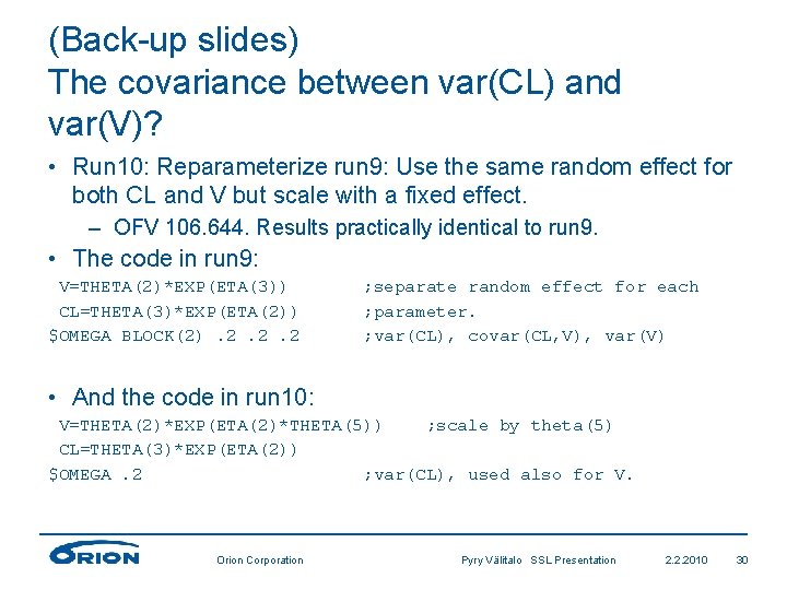
(Back-up slides) The covariance between var(CL) and var(V)? • Run 10: Reparameterize run 9: Use the same random effect for both CL and V but scale with a fixed effect. – OFV 106. 644. Results practically identical to run 9. • The code in run 9: V=THETA(2)*EXP(ETA(3)) CL=THETA(3)*EXP(ETA(2)) $OMEGA BLOCK(2). 2. 2. 2 ; separate random effect for each ; parameter. ; var(CL), covar(CL, V), var(V) • And the code in run 10: V=THETA(2)*EXP(ETA(2)*THETA(5)) ; scale by theta(5) CL=THETA(3)*EXP(ETA(2)) $OMEGA. 2 ; var(CL), used also for V. Orion Corporation Pyry Välitalo SSL Presentation 2. 2. 2010 30

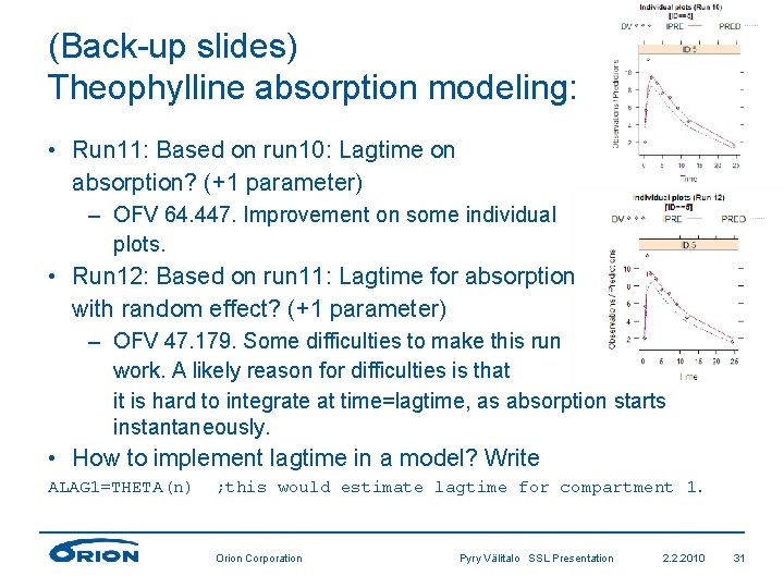
(Back-up slides) Theophylline absorption modeling: • Run 11: Based on run 10: Lagtime on absorption? (+1 parameter) – OFV 64. 447. Improvement on some individual plots. • Run 12: Based on run 11: Lagtime for absorption with random effect? (+1 parameter) – OFV 47. 179. Some difficulties to make this run work. A likely reason for difficulties is that it is hard to integrate at time=lagtime, as absorption starts instantaneously. • How to implement lagtime in a model? Write ALAG 1=THETA(n) ; this would estimate lagtime for compartment 1. Orion Corporation Pyry Välitalo SSL Presentation 2. 2. 2010 31

(Back-up slides) Theophylline absorption modeling • Run 13: Mixed 0 - and 1 st-order absorption – OFV 64. 879 • Run 14: Based on run 13. Mixed 0 - and 1 st-order absorption; a random effect is included for 0 -order absorption rate. – 31. 140. The standard error of var(KA) becomes lower. This seems the most reasonable solution. • How to implement mixed 0 - and 1 st-order absorption? Add a column ”RATE” into the datafile and set it to -2 for every instance when AMT>0 (else ”. ”). Write in the modelfile: D 1=THETA(n) ; this would estimate the duration of a hypothetical ; infusion into the absorption compartment Orion Corporation Pyry Välitalo SSL Presentation 2. 2. 2010 32

(Back-up slides) Absorption phase and residual errors? • Oral dosing data is usually considered more ”noisy” than intravenous dosing data. One reason for this is that despite the best absorption modeling efforts, drug absorption from GI tract can be erratic and/or unpredictable. – Thus, more variability can usually be observed in the absorption phase than in post-absorption phase. • There are instances* when a time-dependent residual error has been assigned to differentiate between absorption phase and post-absorption phase, e. g. IF(T. LE. 2) Y=IPRED+EPS(1) IF(T. GT. 2) Y=IPRED+EPS(2) ; absorption phase, additive error ; post-abs phase, additive error *For example: • Karlsson MO, Beal SL, Sheiner LB. J Pharmacokinet Biopharm. 1995 Dec; 23(6): 651 -72. • Chan PL, Weatherley B, Mc. Fadyen L. Br J Clin Pharmacol. 2008 Apr; 65 Suppl 1: 76 -85. Orion Corporation Pyry Välitalo SSL Presentation 2. 2. 2010 33

(Back-up slides): Runs 15 -16: Test using different residual errors for absorption and post-absorption phases • Run 15: Based on run 10. Try setting the absorption-phase residual error to before 2 hours and post-absorption phase residual error to after 2 hours. – Success: OFV 49. 023, the residual error of post-absorption phase drops to one-half of what it was previously. • Run 16: Based on run 15. Try using proportional residual error for post-absorption phase. – OFV 67. 746. Does not improve the model. Orion Corporation Pyry Välitalo SSL Presentation 2. 2. 2010 34

(Back-up slides): Combine the time-dependent residual error model with absorption model. Implement weight as a covariate. • Run 17: Based on run 14. Combine mixed 0 - and 1 st-order absorption and time-dependent residual error – OFV 19. 804 • Run 18: Based on run 17. Check if a random effect is still needed in the 0 -order absorption rate. – OFV 31. 530 and the standard error of omega(KA) increases. • Runs 19 -22: Try different ways of scaling the volume of distribution and clearance by weight. – Run 20 with linear scaling seems to work best Conclusion: Run 20 shall be the final model. Orion Corporation Pyry Välitalo SSL Presentation 2. 2. 2010 35