A buoyancybased turbulence mixing length technique for cloudless

A buoyancy-based turbulence mixing length technique for cloudless and cloudy boundary layers in the COSMO model Veniamin Perov and Mikhail Chumakov Hydrometcentre of Russia

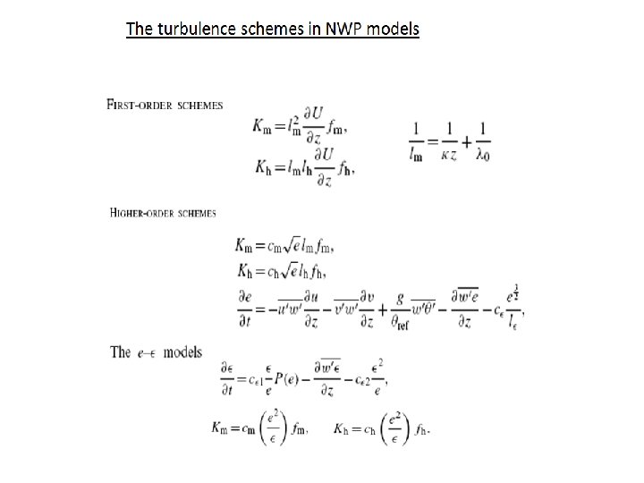
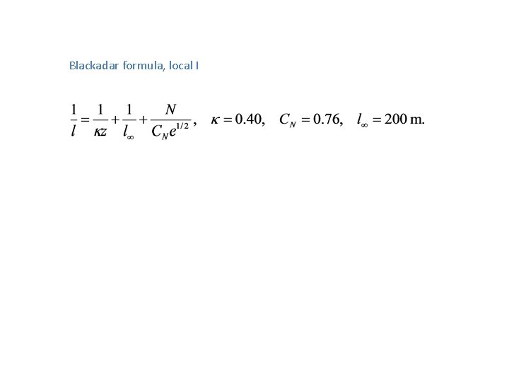
Blackadar formula, local l

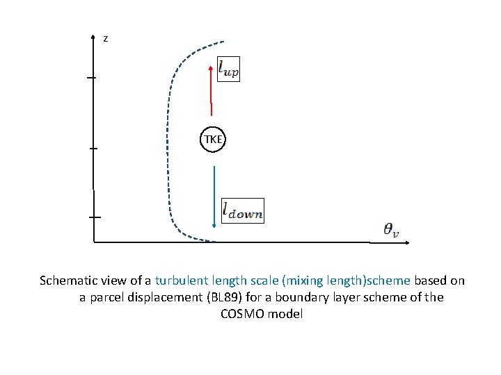
z TKE Schematic view of a turbulent length scale (mixing length)scheme based on a parcel displacement (BL 89) for a boundary layer scheme of the COSMO model

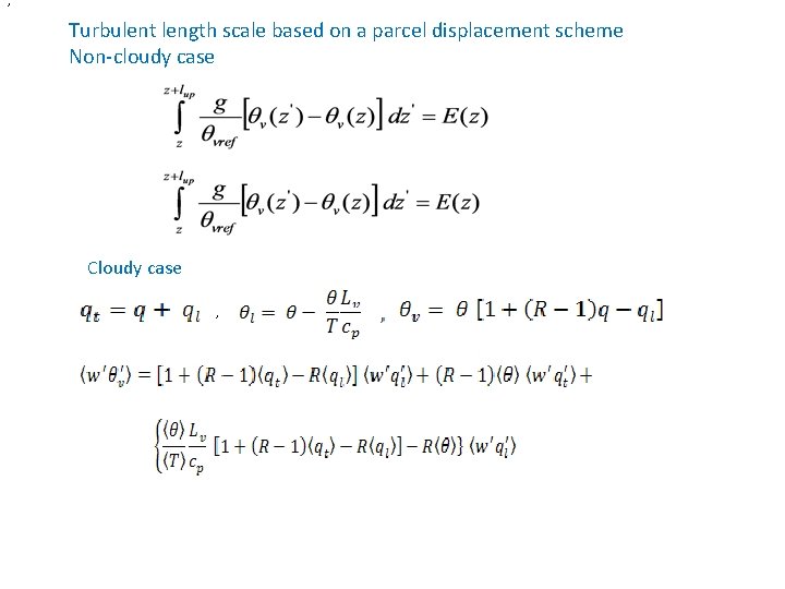
, Turbulent length scale based on a parcel displacement scheme Non-cloudy case Cloudy case ,

Subgrid condensation scheme Calculations of Partial cloudiness in cloudy boundary layers follows Sommeria and Deardorf (1977)

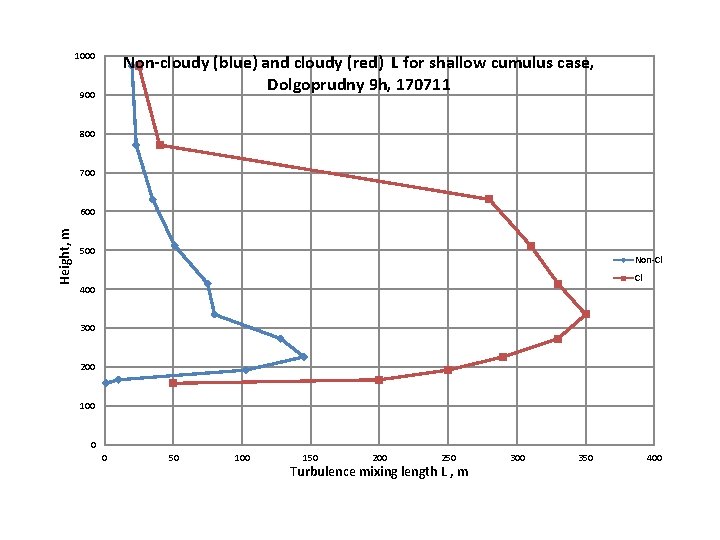
1000 Non-cloudy (blue) and cloudy (red) L for shallow cumulus case, Dolgoprudny 9 h, 170711 900 800 700 Height, m 600 500 Non-Cl Cl 400 300 200 100 0 0 50 100 150 200 250 Turbulence mixing length L , m 300 350 400

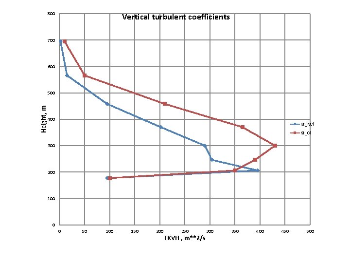
800 Vertical turbulent coefficients 700 600 Height, m 500 400 Kt_NCl Kt_Cl 300 200 100 0 0 50 100 150 200 250 TKVH , m**2/s 300 350 400 450 500

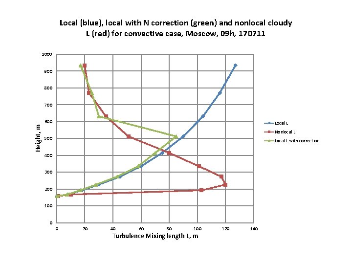
Local (blue), local with N correction (green) and nonlocal cloudy L (red) for convective case, Moscow, 09 h, 170711 1000 900 800 700 Height, m 600 Local L Nonlocal L 500 Local L with correction 400 300 200 100 0 0 20 40 60 80 100 Turbulence Mixing length L, m 120 140

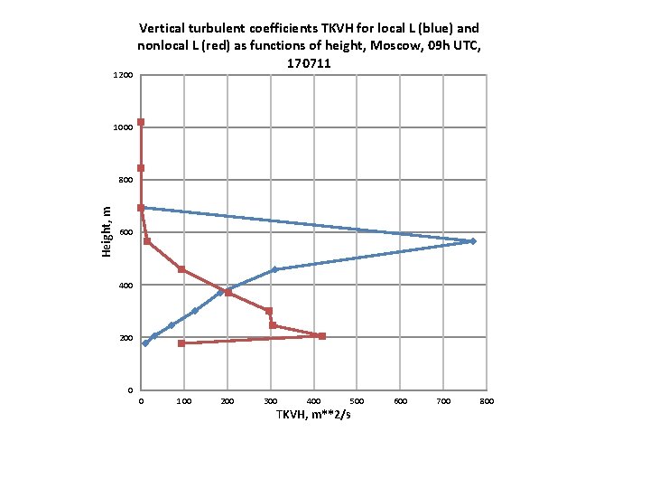
1200 Vertical turbulent coefficients TKVH for local L (blue) and nonlocal L (red) as functions of height, Moscow, 09 h UTC, 170711 1000 Height, m 800 600 400 200 0 0 100 200 300 400 500 TKVH, m**2/s 600 700 800

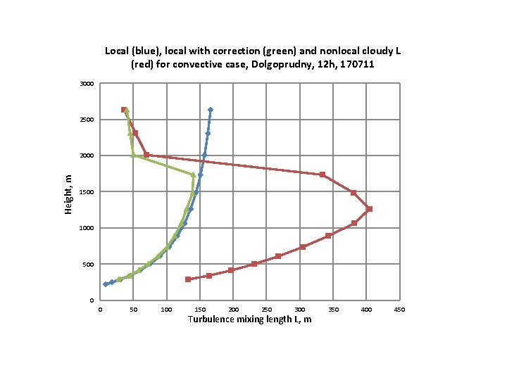
Local (blue), local with correction (green) and nonlocal cloudy L (red) for convective case, Dolgoprudny, 12 h, 170711 3000 2500 Height, m 2000 1500 1000 500 0 0 50 100 150 200 250 300 Turbulence mixing length L, m 350 400 450

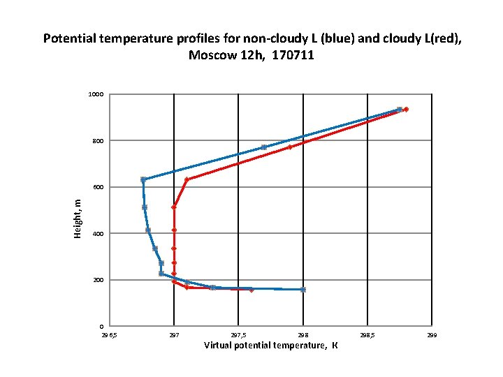
Potential temperature profiles for non-cloudy L (blue) and cloudy L(red), Moscow 12 h, 170711 1000 800 Height, m 600 400 200 0 296, 5 297, 5 298 Virtual potential temperature, К 298, 5 299

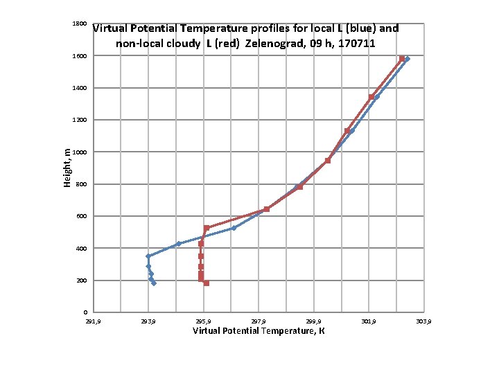
1800 Virtual Potential Temperature profiles for local L (blue) and non-local cloudy L (red) Zelenograd, 09 h, 170711 1600 1400 Height, m 1200 1000 800 600 400 200 0 291, 9 293, 9 295, 9 297, 9 299, 9 Virtual Potential Temperature, К 301, 9 303, 9

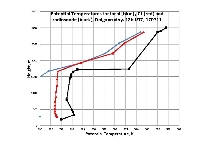
3500 Potential Temperatures for local (blue) , CL (red) and radiosonde (black), Dolgoprudny, 12 h UTC, 170711 3000 Height, m 2500 2000 1500 1000 500 0 295 296 297 298 299 300 301 302 303 Potential Temperature, K 304 305 306 307 308

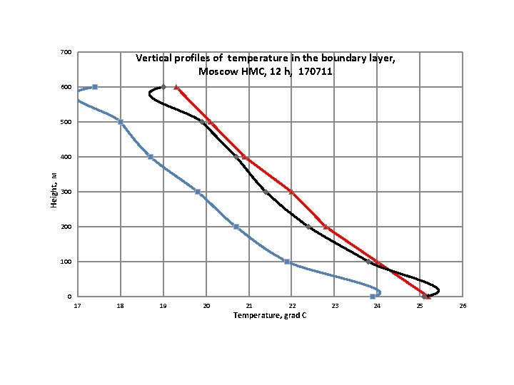
700 Vertical profiles of temperature in the boundary layer, Moscow HMC, 12 h, 170711 600 500 Height, м 400 300 200 100 0 17 18 19 20 21 22 Temperature, grad С 23 24 25 26

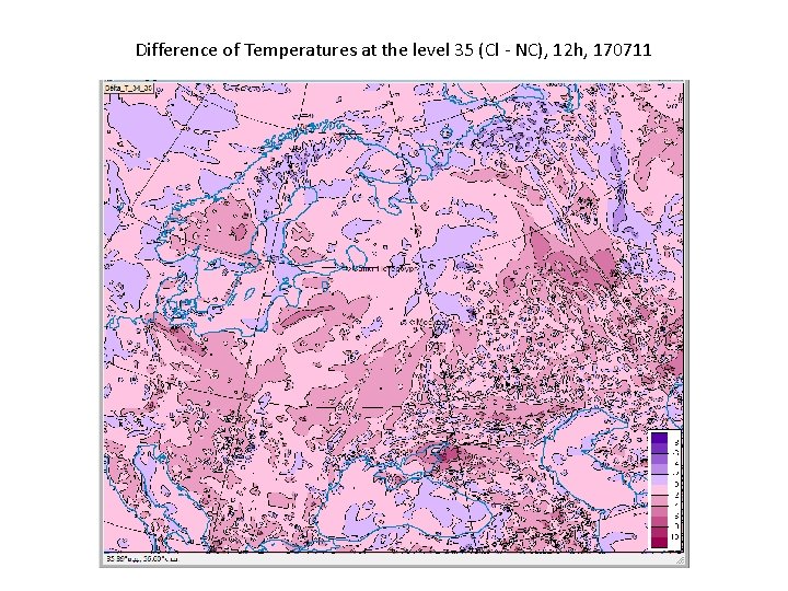
Difference of Temperatures at the level 35 (Cl - NC), 12 h, 170711

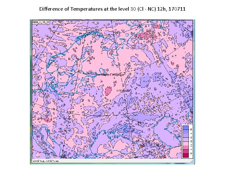
Difference of Temperatures at the level 30 (Cl - NC) 12 h, 170711

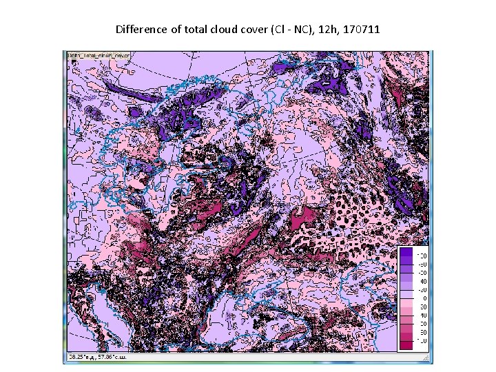
Difference of total cloud cover (Cl - NC), 12 h, 170711

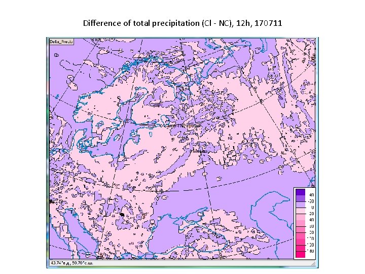
Difference of total precipitation (Cl - NC), 12 h, 170711

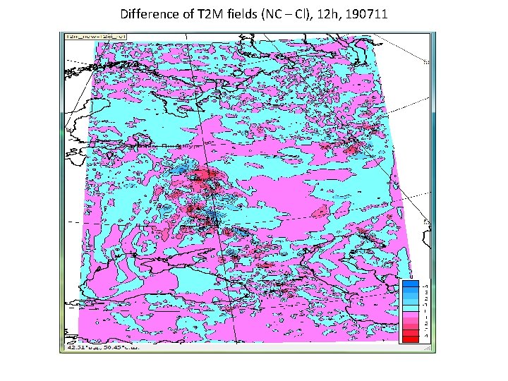
Difference of T 2 M fields (NC – Cl), 12 h, 190711

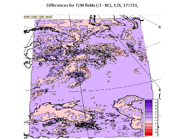
Differences for T 2 M fields (Cl - NC), 12 h, 170711,

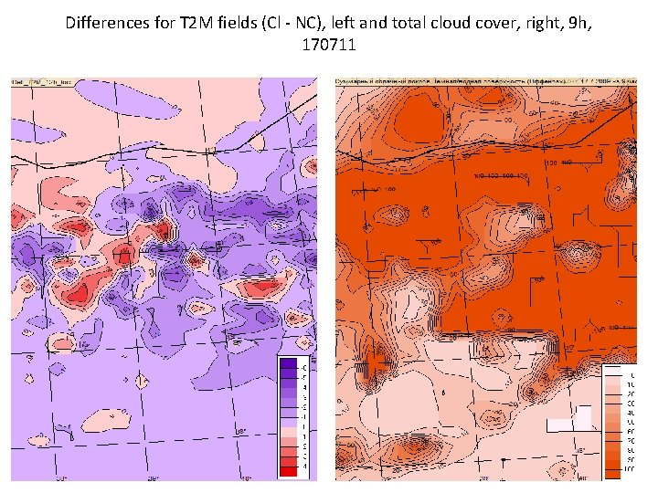
Differences for T 2 M fields (Cl - NC), left and total cloud cover, right, 9 h, 170711

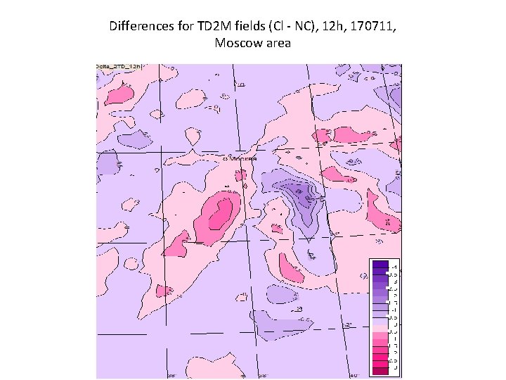
Differences for TD 2 M fields (Cl - NC), 12 h, 170711, Moscow area

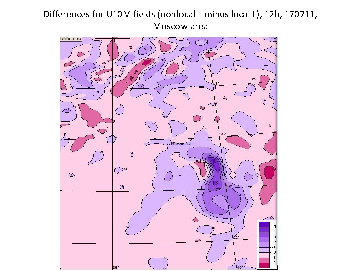
Differences for U 10 M fields (nonlocal L minus local L), 12 h, 170711, Moscow area

Main results • Algorithm for computing the nonlinear turbulence length scale based on displacement method of air parcel (BL 89) was developed for cloudy boundary layers. A new algorithm for calculation turbulence length scale has a more rigorous physical basis in comparison with the algorithm for dry boundary layers and currently used (Blackadar formulae). • Algorithm was impact in module TUBDIFF of main COSMO program • Calculations were performed for convective situations (July 2009) by full 3 -D COSMO model (version 4. 13). Results showed differences in fields of temperature, humidity, clouds and wind between variants with L for cloudy boundary layers and L for non-cloudy BL.

Thank you for your attention!

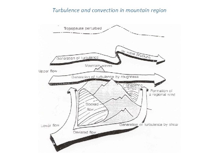
Turbulence and convection in mountain region

Mesoscale modeling in mountain region • Mesoscale modeling in mountain area should include simulations of main processes in this domain. These are formation of the regional slope winds, blocked flow, deviated flow, sheltering effect after obstacle, generation of turbulence by wind shear at the lower part of flow. • In the upper part of flow it will be generation of turbulence by roughness, mountain waves and generation of turbulence by mountain wave breaking. • For high mountains we need also to take into account a tropopause perturbation. All these processes require the use of three-dimensional turbulence and the non-use of simple diagnostic formulas for turbulence length scale (mixing length). • In this case, together with the equation for the turbulent kinetic energy (TKE) will have to use the equation for mixing length ( for example equation for dissipation of TKE).

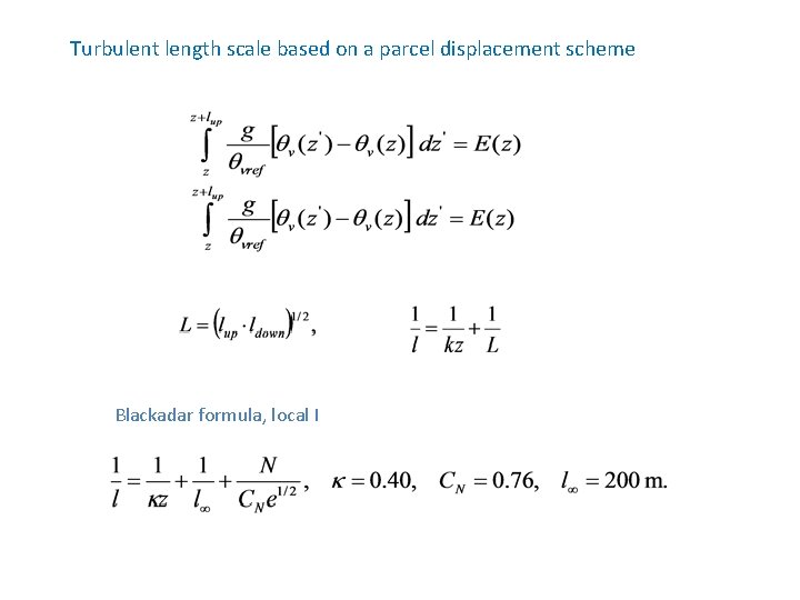
Turbulent length scale based on a parcel displacement scheme Blackadar formula, local l