A brief survey of the LAMMPS particle simulation

A brief survey of the LAMMPS particle simulation code: introduction, case studies, and future development Paul S. Crozier August 10, 2011 Sandia National Laboratories is a multi-program laboratory managed and operated by Sandia Corporation, a wholly owned subsidiary of Lockheed Martin Corporation, for the U. S. Department of Energy’s National Nuclear Security Administration under contract DE-AC 04 -94 AL 85000.

Acknowledgements Steve Plimpton (1426) Aidan Thompson (1425) Many other contributors to LAMMPS (see: http: //lammps. sandia. gov/authors. html)

Discussion outline 1. 2. 3. 4. 5. 6. 7. 8. 9. 10. 11. MD basics Why use LAMMPS? Live demo #1 Basic information about LAMMPS Live demo #2 Six very useful LAMMPS commands Live demo #3 Vignettes of some LAMMPS research Future areas of LAMMPS development How to add a new feature to LAMMPS Homework assignment

Review of MD basics • MD: molecular dynamics • F = ma • Classical dynamics • Rapidly grown in popularity and use in research • Computationally intensive, especially computation of nonbonded interactions • Uses force fields: mathematical models of interatomic interactions

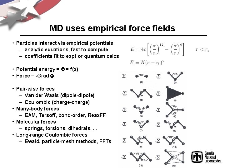
MD uses empirical force fields • Particles interact via empirical potentials – analytic equations, fast to compute – coefficients fit to expt or quantum calcs • Potential energy = = f(x) • Force = -Grad • Pair-wise forces – Van der Waals (dipole-dipole) – Coulombic (charge-charge) • Many-body forces – EAM, Tersoff, bond-order, Reax. FF • Molecular forces – springs, torsions, dihedrals, . . . • Long-range Coulombic forces – Ewald, particle-mesh methods, FFTs

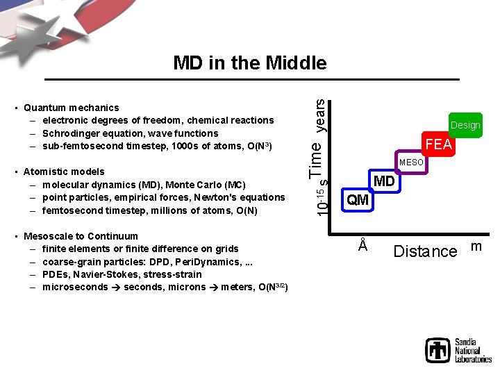
• Quantum mechanics – electronic degrees of freedom, chemical reactions – Schrodinger equation, wave functions – sub-femtosecond timestep, 1000 s of atoms, O(N 3) • Atomistic models – molecular dynamics (MD), Monte Carlo (MC) – point particles, empirical forces, Newton's equations – femtosecond timestep, millions of atoms, O(N) • Mesoscale to Continuum – finite elements or finite difference on grids – coarse-grain particles: DPD, Peri. Dynamics, . . . – PDEs, Navier-Stokes, stress-strain – microseconds seconds, microns meters, O(N 3/2) 10 -15 s. Time years MD in the Middle Design FEA MESO MD QM Å Distance m

Algorithmic Issues in MD • Speed – parallel implementation • Accuracy – long-range Coulombics • Time scale – slow versus fast degrees of freedom • Length scale – coarse-graining

Classical MD in Parallel • MD is inherently parallel – forces on each atom can be computed simultaneously – X and V can be updated simultaneously • Most MD codes are parallel – via distributed-memory message-passing paradigm (MPI) • Computation scales as N = number of atoms – ideally would scale as N/P in parallel • Can distribute: – atoms – forces – space communication = scales as N/sqrt(P) communication = scales as N/P or (N/P)2/3

Discussion outline 1. 2. 3. 4. 5. 6. 7. 8. 9. 10. 11. MD basics Why use LAMMPS? Live demo #1 Basic information about LAMMPS Live demo #2 Six very useful LAMMPS commands Live demo #3 Vignettes of some LAMMPS research Future areas of LAMMPS development How to add a new feature to LAMMPS Homework assignment

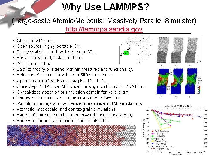
Why Use LAMMPS? (Large-scale Atomic/Molecular Massively Parallel Simulator) http: //lammps. sandia. gov § § § § Classical MD code. Open source, highly portable C++. Freely available for download under GPL. Easy to download, install, and run. Well documented. Easy to modify or extend with new features and functionality. Active user’s e-mail list with over 650 subscribers. Upcoming users’ workshop: Aug 9 – 11, 2011. Since Sept. 2004: over 50 k downloads, grown from 53 to 175 kloc. Spatial-decomposition of simulation domain for parallelism. Energy minimization via conjugate-gradient relaxation. Radiation damage and two temperature model (TTM) simulations. Atomistic, mesoscale, and coarse-grain simulations. Variety of potentials (including many-body and coarse-grain). Variety of boundary conditions, constraints, etc.

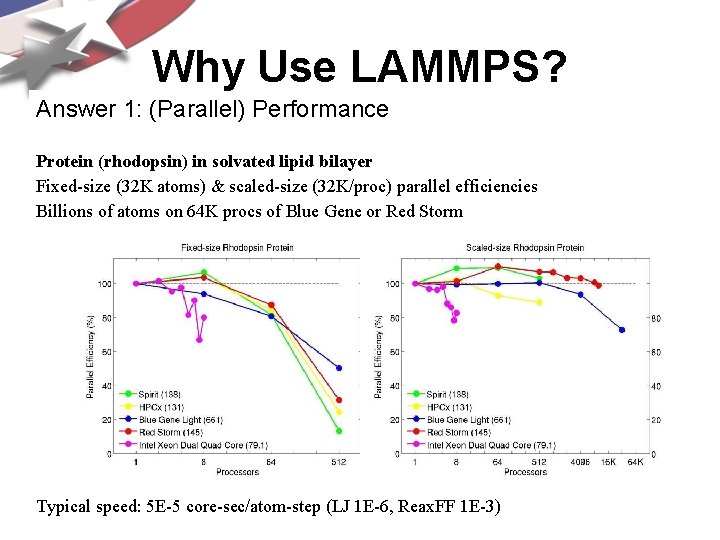
Why Use LAMMPS? Answer 1: (Parallel) Performance Protein (rhodopsin) in solvated lipid bilayer Fixed-size (32 K atoms) & scaled-size (32 K/proc) parallel efficiencies Billions of atoms on 64 K procs of Blue Gene or Red Storm Typical speed: 5 E-5 core-sec/atom-step (LJ 1 E-6, Reax. FF 1 E-3)

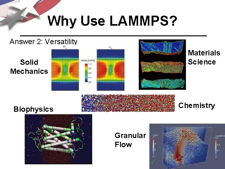
Why Use LAMMPS? Answer 2: Versatility Materials Science Solid Mechanics Chemistry Biophysics Granular Flow

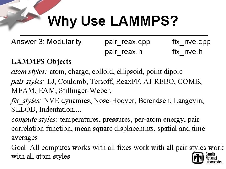
Why Use LAMMPS? Answer 3: Modularity pair_reax. cpp pair_reax. h fix_nve. cpp fix_nve. h LAMMPS Objects atom styles: atom, charge, colloid, ellipsoid, point dipole pair styles: LJ, Coulomb, Tersoff, Reax. FF, AI-REBO, COMB, MEAM, Stillinger-Weber, fix_styles: NVE dynamics, Nose-Hoover, Berendsen, Langevin, SLLOD, Indentation, . . . compute styles: temperatures, pressures, per-atom energy, pair correlation function, mean square displacemnts, spatial and time averages Goal: All computes works with all fixes work with all pair styles work with all atom styles

Why Use LAMMPS? Answer 4: Potential Coverage LAMMPS Potentials pairwise potentials: Lennard-Jones, Buckingham, . . . charged pairwise potentials: Coulombic, point-dipole manybody potentials: EAM, Finnis/Sinclair, modified EAM (MEAM), embedded ion method (EIM), Stillinger-Weber, Tersoff, AI -REBO, Reax. FF, COMB electron force field (e. FF) coarse-grained potentials: DPD, Gay. Berne, . . . mesoscopic potentials: granular, peridynamics long-range Coulombics and dispersion: Ewald, PPPM (similar to particle-mesh Ewald)

Why Use LAMMPS? Answer 4: Potentials LAMMPS Potentials (contd. ) bond potentials: harmonic, FENE, . . . angle potentials: harmonic, CHARMM, . . . dihedral potentials: harmonic, CHARMM, . . . improper potentials: harmonic, cvff, class 2 (COMPASS) polymer potentials: all-atom, united-atom, bead-spring, breakable water potentials: TIP 3 P, TIP 4 P, SPC implicit solvent potentials: hydrodynamic lubrication, Debye force-field compatibility with common CHARMM, AMBER, OPLS, GROMACS options

Why Use LAMMPS? Answer 4: Range of Potentials LAMMPS Potentials Biomolecules: CHARMM, AMBER, OPLS, COMPASS (class 2), long-range Coulombics via PPPM, point dipoles, . . . Polymers: all-atom, united-atom, coarse-grain (bead-spring FENE), bond-breaking, … Materials: EAM and MEAM for metals, Buckingham, Morse, Yukawa, Stillinger-Weber, Tersoff, AI-REBO, Reax. FF, COMB, e. FF. . . Mesoscale: granular, DPD, Gay-Berne, colloidal, peri-dynamics, DSMC. . . Hybrid: can use combinations of potentials for hybrid systems: water on metal, polymers/semiconductor interface, colloids in solution, …

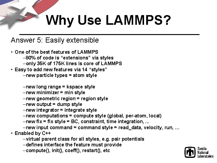
Why Use LAMMPS? Answer 5: Easily extensible • One of the best features of LAMMPS – 80% of code is “extensions” via styles –only 35 K of 175 K lines is core of LAMMPS • Easy to add new features via 14 “styles” –new particle types = atom style –new force fields = pair style, bond style, angle style, dihedral style, improper style –new long range = kspace style –new minimizer = min style –new geometric region = region style –new output = dump style –new integrator = integrate style –new computations = compute style (global, per-atom, local) –new fix = fix style = BC, constraint, time integration, . . . –new input command = command style = read_data, velocity, run, … • Enabled by C++ –virtual parent class for all styles, e. g. pair potentials –defines interface the feature must provide –compute(), init(), coeff(), restart(), etc

How to download, install, and use LAMMPS • Download page: lammps. sandia. gov/download. html • Installation instructions: lammps. sandia. gov/doc/Section_start. html go to lammps/src type “make your_system_type” • To perform a simulation: lmp < my_script. in

Live demo #1 1. Download LAMMPS. – – http: //lammps. sandia. gov/download. html Try the Windows serial executable. 2. Download a simple LAMMPS input script. – http: //lammps. sandia. gov/inputs/in. lj. txt 3. Run LAMMPS – http: //lammps. sandia. gov/doc/Section_start. html#2_5

Discussion outline 1. 2. 3. 4. 5. 6. 7. 8. 9. 10. 11. MD basics Why use LAMMPS? Live demo #1 Basic information about LAMMPS Live demo #2 Six very useful LAMMPS commands Live demo #3 Vignettes of some LAMMPS research Future areas of LAMMPS development How to add a new feature to LAMMPS Homework assignment

How to get help with LAMMPS 1. Excellent User’s Manual: http: //lammps. sandia. gov/doc/Manual. html http: //lammps. sandia. gov/doc/Section_commands. html#3_5 2. Search the web: can include “lammps-users” as a search keyword to search old e-mail archives 3. Send e-mail to the user’s e-mail list: http: //lammps. sandia. gov/mail. html 4. Contact LAMMPS developers: http: //lammps. sandia. gov/authors. html Steve Plimpton, sjplimp@sandia. gov Aidan Thompson, athomps@sandia. gov Paul Crozier, pscrozi@sandia. gov

Force fields available in LAMMPS • Biomolecules: CHARMM, AMBER, OPLS, COMPASS (class 2), long-range Coulombics via PPPM, point dipoles, . . . • Polymers: all-atom, united-atom, coarse-grain (bead-spring FENE), bond-breaking, … • Materials: EAM and MEAM for metals, Buckingham, Morse, Yukawa, Stillinger-Weber, Tersoff, AI-REBO, Reaxx FF, . . . • Mesoscale: granular, DPD, Gay-Berne, colloidal, peri-dynamics, DSMC. . . • Hybrid: can use combinations of potentials for hybrid systems: water on metal, polymers/semiconductor interface, colloids in solution, …

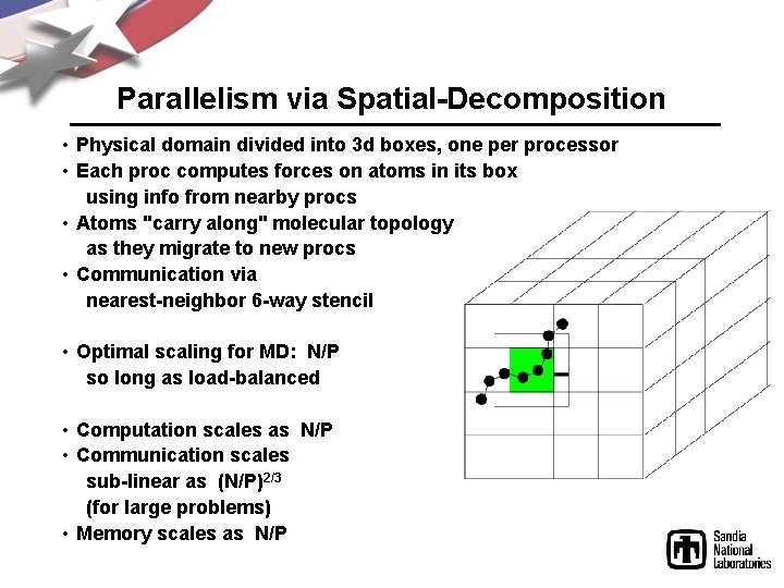
Parallelism via Spatial-Decomposition • Physical domain divided into 3 d boxes, one per processor • Each proc computes forces on atoms in its box using info from nearby procs • Atoms "carry along" molecular topology as they migrate to new procs • Communication via nearest-neighbor 6 -way stencil • Optimal scaling for MD: N/P so long as load-balanced • Computation scales as N/P • Communication scales sub-linear as (N/P)2/3 (for large problems) • Memory scales as N/P

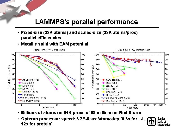
LAMMPS’s parallel performance • Fixed-size (32 K atoms) and scaled-size (32 K atoms/proc) parallel efficiencies • Metallic solid with EAM potential • Billions of atoms on 64 K procs of Blue Gene or Red Storm • Opteron processor speed: 5. 7 E-6 sec/atom/step (0. 5 x for LJ, 12 x for protein)

Easily add your own LAMMPS feature • New user or new simulation always want new feature not in code • Goal: make it as easy as possible for us and others to add new features called “styles” in LAMMPS: particle type, pair or bond potential, scalar or per-atom computation "fix": BC, force constraint, time integration, diagnostic, . . . input command: create_atoms, set, run, temper, . . . over 75% of current 170 K+ lines of LAMMPS is add-on styles • Enabled by C++ "virtual" parent class for all pair potentials defines interface: compute(), coeff(), restart(), . . . add feature: add 2 lines to header file, add files to src dir, re-compile feature won't exist if not used, won't conflict with rest of code • Of course, someone has to write the code for the feature!

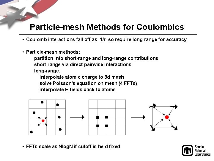
Particle-mesh Methods for Coulombics • Coulomb interactions fall off as 1/r so require long-range for accuracy • Particle-mesh methods: partition into short-range and long-range contributions short-range via direct pairwise interactions long-range: interpolate atomic charge to 3 d mesh solve Poisson's equation on mesh (4 FFTs) interpolate E-fields back to atoms • FFTs scale as Nlog. N if cutoff is held fixed

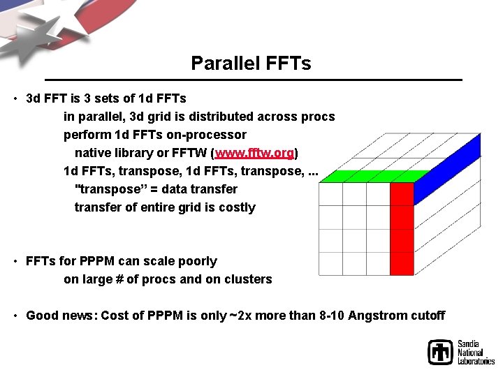
Parallel FFTs • 3 d FFT is 3 sets of 1 d FFTs in parallel, 3 d grid is distributed across procs perform 1 d FFTs on-processor native library or FFTW (www. fftw. org) 1 d FFTs, transpose, . . . "transpose” = data transfer of entire grid is costly • FFTs for PPPM can scale poorly on large # of procs and on clusters • Good news: Cost of PPPM is only ~2 x more than 8 -10 Angstrom cutoff

Time Scale of Molecular Dynamics • Limited timescale is most serious drawback of MD • Timestep size limited by atomic oscillations: – C-H bond = 10 fmsec ½ to 1 fmsec timestep – Debye frequency = 1013 2 fmsec timestep • A state-of-the-art “long” simulation is nanoseconds to a microsecond of real time • Reality is usually on a much longer timescale: – protein folding (msec to seconds) – polymer entanglement (msec and up) – glass relaxation (seconds to decades)

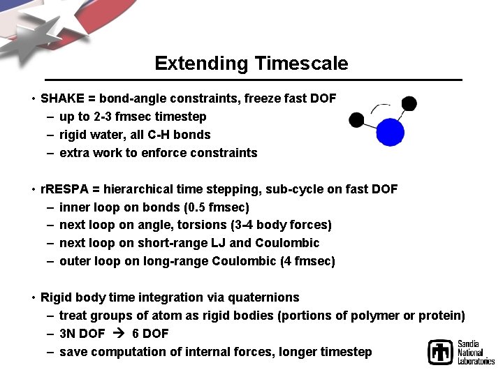
Extending Timescale • SHAKE = bond-angle constraints, freeze fast DOF – up to 2 -3 fmsec timestep – rigid water, all C-H bonds – extra work to enforce constraints • r. RESPA = hierarchical time stepping, sub-cycle on fast DOF – inner loop on bonds (0. 5 fmsec) – next loop on angle, torsions (3 -4 body forces) – next loop on short-range LJ and Coulombic – outer loop on long-range Coulombic (4 fmsec) • Rigid body time integration via quaternions – treat groups of atom as rigid bodies (portions of polymer or protein) – 3 N DOF 6 DOF – save computation of internal forces, longer timestep

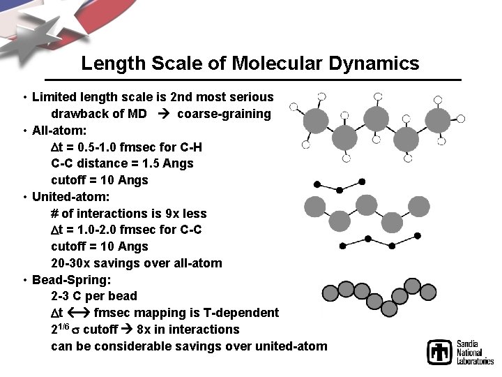
Length Scale of Molecular Dynamics • Limited length scale is 2 nd most serious drawback of MD coarse-graining • All-atom: t = 0. 5 -1. 0 fmsec for C-H C-C distance = 1. 5 Angs cutoff = 10 Angs • United-atom: # of interactions is 9 x less t = 1. 0 -2. 0 fmsec for C-C cutoff = 10 Angs 20 -30 x savings over all-atom • Bead-Spring: 2 -3 C per bead t fmsec mapping is T-dependent 21/6 cutoff 8 x in interactions can be considerable savings over united-atom

Live demo #2 1. Modify the input script from live demo #1 – Add the line “dump 1 all atom 10 atoms. lammpstrj” between the fix and run command lines. 2. Run LAMMPS with the modified input script. 3. Visualize the simulation results using 3 rd party software (VMD) – – – http: //www. ks. uiuc. edu/Research/vmd/ Start up VMD and open the “atoms. lammpstrj” file View the “movie” you’ve made from the LAMMPS trajectory by pressing the play button.

Discussion outline 1. 2. 3. 4. 5. 6. 7. 8. 9. 10. 11. MD basics Why use LAMMPS? Live demo #1 Basic information about LAMMPS Live demo #2 Six very useful LAMMPS commands Live demo #3 Vignettes of some LAMMPS research Future areas of LAMMPS development How to add a new feature to LAMMPS Homework assignment

Six very useful LAMMPS commands 1. 2. 3. 4. 5. 6. fix compute pair_style variable thermo_style dump

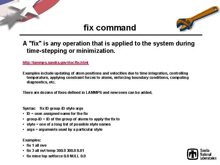
fix command A "fix" is any operation that is applied to the system during time-stepping or minimization. http: //lammps. sandia. gov/doc/fix. html Examples include updating of atom positions and velocities due to time integration, controlling temperature, applying constraint forces to atoms, enforcing boundary conditions, computing diagnostics, etc. There are dozens of fixes defined in LAMMPS and new ones can be added. Syntax: fix ID group-ID style args • ID = user-assigned name for the fix • group-ID = ID of the group of atoms to apply the fix to • style = one of a long list of possible style names • args = arguments used by a particular style Examples: • fix 1 all nve • fix 3 all nvt temp 300. 01 • fix mine top setforce 0. 0 NULL 0. 0

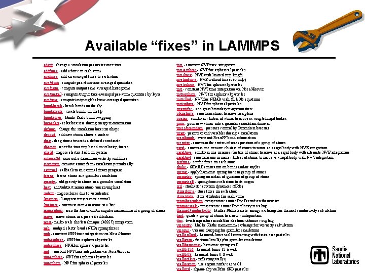
Available “fixes” in LAMMPS adapt - change a simulation parameter over time addforce - add a force to each atom aveforce - add an averaged force to each atom ave/atom - compute per-atom time-averaged quantities ave/histo - compute/output time-averaged histograms ave/spatial - compute/output time-averaged per-atom quantities by layer ave/time - compute/output global time-averaged quantities bond/break - break bonds on the fly bond/create - create bonds on the fly bond/swap - Monte Carlo bond swapping box/relax - relax box size during energy minimization deform - change the simulation box size/shape deposit - add new atoms above a surface drag - drag atoms towards a defined coordinate dt/reset - reset the timestep based on velocity, forces efield - impose electric field on system enforce 2 d - zero out z-dimension velocity and force evaporate - remove atoms from simulation periodically external - callback to an external driver program freeze - freeze atoms in a granular simulation gravity - add gravity to atoms in a granular simulation heat - add/subtract momentum-conserving heat indent - impose force due to an indenter langevin - Langevin temperature control lineforce - constrain atoms to move in a line momentum - zero the linear and/or angular momentum of a group of atoms move - move atoms in a prescribed fashion msst - multi-scale shock technique (MSST) integration neb - nudged elastic band (NEB) spring forces nph - constant NPH time integration via Nose/Hoover nph/asphere - NPH for aspherical particles nph/sphere - NPH for spherical particles npt - constant NPT time integration via Nose/Hoover npt/asphere - NPT for aspherical particles npt/sphere - NPT for spherical particles nve - constant NVE time integration nve/asphere - NVT for aspherical particles nve/limit - NVE with limited step length nve/noforce - NVE without forces (v only) nve/sphere - NVT for spherical particles nvt - constant NVT time integration via Nose/Hoover nvt/asphere - NVT for aspherical particles nvt/sllod - NVT for NEMD with SLLOD equations nvt/sphere - NVT for spherical particles orient/fcc - add grain boundary migration force planeforce - constrain atoms to move in a plane poems - constrain clusters of atoms to move as coupled rigid bodies pour - pour new atoms into a granular simulation domain press/berendsen - pressure control by Berendsen barostat print - print text and variables during a simulation reax/bonds - write out Reax. FF bond information recenter - constrain the center-of-mass position of a group of atoms rigid - constrain one or more clusters of atoms to move as a rigid body with NVE integration rigid/nve - constrain one or more clusters of atoms to move as a rigid body with alternate NVE integration rigid/nvt - constrain one or more clusters of atoms to move as a rigid body with NVT integration setforce - set the force on each atom shake - SHAKE constraints on bonds and/or angles spring - apply harmonic spring force to group of atoms spring/rg - spring on radius of gyration of group of atoms spring/self - spring from each atom to its origin srd - stochastic rotation dynamics (SRD) store/force - store force on each atom store/state - store attributes for each atom temp/berendsen - temperature control by Berendsen thermostat temp/rescale - temperature control by velocity rescaling thermal/conductivity - Muller-Plathe kinetic energy exchange for thermal conductivity calculation tmd - guide a group of atoms to a new configuration ttm - two-temperature model for electronic/atomic coupling viscosity - Muller-Plathe momentum exchange for viscosity calculation viscous - viscous damping for granular simulations wall/colloid - Lennard-Jones wall interacting with finite-size particles wall/gran - frictional wall(s) for granular simulations wall/harmonic - harmonic spring wall/lj 126 - Lennard-Jones 12 -6 wall/lj 93 - Lennard-Jones 9 -3 wall/reflect - reflecting wall(s) wall/region - use region surface as wall/srd - slip/no-slip wall for SRD particles

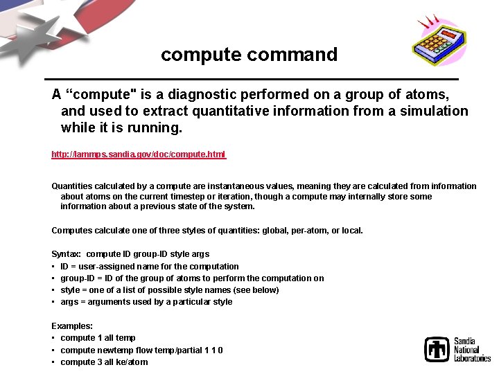
compute command A “compute" is a diagnostic performed on a group of atoms, and used to extract quantitative information from a simulation while it is running. http: //lammps. sandia. gov/doc/compute. html Quantities calculated by a compute are instantaneous values, meaning they are calculated from information about atoms on the current timestep or iteration, though a compute may internally store some information about a previous state of the system. Computes calculate one of three styles of quantities: global, per-atom, or local. Syntax: compute ID group-ID style args • ID = user-assigned name for the computation • group-ID = ID of the group of atoms to perform the computation on • style = one of a list of possible style names (see below) • args = arguments used by a particular style Examples: • compute 1 all temp • compute newtemp flow temp/partial 1 1 0 • compute 3 all ke/atom

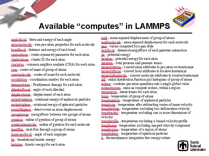
Available “computes” in LAMMPS angle/local - theta and energy of each angle atom/molecule - sum per-atom properties for each molecule bond/local - distance and energy of each bond centro/atom - centro-symmetry parameter for each atom cluster/atom - cluster ID for each atom cna/atom - common neighbor analysis (CNA) for each atom com - center-of-mass of group of atoms com/molecule - center-of-mass for each molecule coord/atom - coordination number for each atom damage/atom - Peridynamic damage for each atom dihedral/local - angle of each dihedral displace/atom - displacement of each atom erotate/asphere - rotational energy of aspherical particles erotate/sphere - rotational energy of spherical particles event/displace - detect event on atom displacement group/group - energy/force between two groups of atoms gyration - radius of gyration of group of atoms gyration/molecule - radius of gyration for each molecule heat/flux - heat flux through a group of atoms improper/local - angle of each improper ke - translational kinetic energy ke/atom - kinetic energy for each atom msd - mean-squared displacement of group of atoms msd/molecule - mean-squared displacement for each molecule pair - values computed by a pair style pair/local - distance/energy/force of each pairwise interaction pe - potential energy pe/atom - potential energy for each atom pressure - total pressure and pressure tensor property/atom - convert atom attributes to per-atom vectors/arrays property/local - convert local attributes to localvectors/arrays property/molecule - convert molecule attributes to localvectors/arrays rdf - radial distribution function g(r) histogram of group of atoms reduce - combine per-atom quantities into a single global value reduce/region - same as compute reduce, within a region stress/atom - stress tensor for each atom temp - temperature of group of atoms temp/asphere - temperature of aspherical particles temp/com - temperature after subtracting center-of-mass velocity temp/deform - temperature excluding box deformation velocity temp/partial - temperature excluding one or more dimensions of velocity temp/profile - temperature excluding a binned velocity profile temp/ramp - temperature excluding ramped velocity component temp/region - temperature of a region of atoms temp/sphere - temperature of spherical particles ti - thermodyanmic integration free energy values

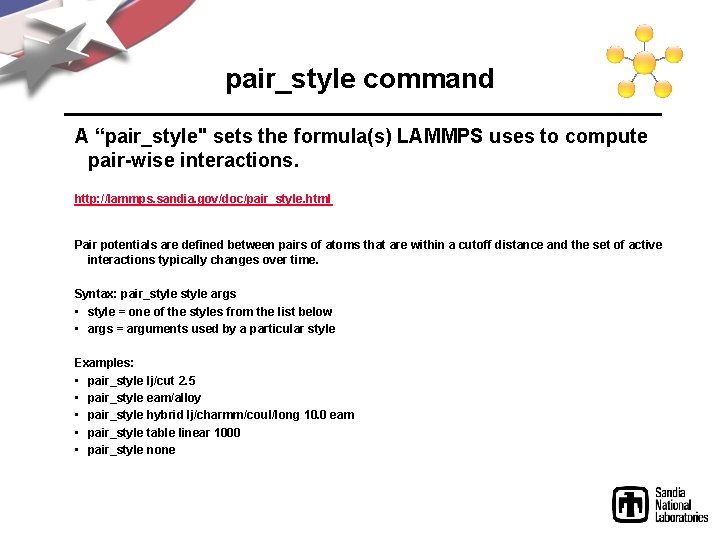
pair_style command A “pair_style" sets the formula(s) LAMMPS uses to compute pair-wise interactions. http: //lammps. sandia. gov/doc/pair_style. html Pair potentials are defined between pairs of atoms that are within a cutoff distance and the set of active interactions typically changes over time. Syntax: pair_style args • style = one of the styles from the list below • args = arguments used by a particular style Examples: • pair_style lj/cut 2. 5 • pair_style eam/alloy • pair_style hybrid lj/charmm/coul/long 10. 0 eam • pair_style table linear 1000 • pair_style none

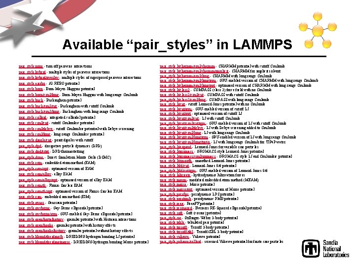
Available “pair_styles” in LAMMPS pair_style none - turn off pairwise interactions pair_style hybrid - multiple styles of pairwise interactions pair_style hybrid/overlay - multiple styles of superposed pairwise interactions pair_style airebo - AI-REBO potential pair_style born - Born-Mayer-Huggins potential pair_style born/coul/long - Born-Mayer-Huggins with long-range Coulomb pair_style buck - Buckingham potential pair_style buck/coul/cut - Buckingham with cutoff Coulomb pair_style buck/coul/long - Buckingham with long-range Coulomb pair_style colloid - integrated colloidal potential pair_style coul/cut - cutoff Coulombic potential pair_style coul/debye - cutoff Coulombic potential with Debye screening pair_style coul/long - long-range Coulombic potential pair_style dipole/cut - point dipoles with cutoff pair_style dpd - dissipative particle dynamics (DPD) pair_style dpd/tstat - DPD thermostatting pair_style dsmc - Direct Simulation Monte Carlo (DSMC) pair_style eam - embedded atom method (EAM) pair_style eam/opt - optimized version of EAM pair_style eam/alloy - alloy EAM pair_style eam/alloy/opt - optimized version of alloy EAM pair_style eam/fs - Finnis-Sinclair EAM pair_style eam/fs/opt - optimized version of Finnis-Sinclair EAM pair_style eim - embedded ion method (EIM) pair_style gauss - Gaussian potential pair_style gayberne - Gay-Berne ellipsoidal potential pair_style gayberne/gpu - GPU-enabled Gay-Berne ellipsoidal potential pair_style gran/hertz/history - granular potential with Hertzian interactions pair_style gran/hooke - granular potential with history effects pair_style gran/hooke/history - granular potential without history effects pair_style hbond/dreiding/lj - DREIDING hydrogen bonding LJ potential pair_style hbond/dreiding/morse - DREIDING hydrogen bonding Morse potential pair_style lj/charmm/coul/charmm - CHARMM potential with cutoff Coulomb pair_style lj/charmm/coul/charmm/implicit - CHARMM for implicit solvent pair_style lj/charmm/coul/long - CHARMM with long-range Coulomb pair_style lj/charmm/coul/long/gpu - GPU-enabled version of CHARMM with long-range Coulomb pair_style lj/charmm/coul/long/opt - optimized version of CHARMM with long-range Coulomb pair_style lj/class 2 - COMPASS (class 2) force field with no Coulomb pair_style lj/class 2/coul/cut - COMPASS with cutoff Coulomb pair_style lj/class 2/coul/long - COMPASS with long-range Coulomb pair_style lj/cut - cutoff Lennard-Jones potential with no Coulomb pair_style lj/cut/gpu - GPU-enabled version of cutoff LJ pair_style lj/cut/opt - optimized version of cutoff LJ pair_style lj/cut/coul/cut - LJ with cutoff Coulomb pair_style lj/cut/coul/cut/gpu - GPU-enabled version of LJ with cutoff Coulomb pair_style lj/cut/coul/debye - LJ with Debye screening added to Coulomb pair_style lj/cut/coul/long - LJ with long-range Coulomb pair_style lj/cut/coul/long/gpu - GPU-enabled version of LJ with long-range Coulomb pair_style lj/cut/coul/long/tip 4 p - LJ with long-range Coulomb for TIP 4 P water pair_style lj/expand - Lennard-Jones for variable size particles pair_style lj/gromacs - GROMACS-style Lennard-Jones potential pair_style lj/gromacs/coul/gromacs - GROMACS-style LJ and Coulombic potential pair_style lj/smooth - smoothed Lennard-Jones potential pair_style lj 96/cut - Lennard-Jones 9/6 potential pair_style lj 96/cut/gpu - GPU-enabled version of Lennard-Jones 9/6 pair_style lubricate - hydrodynamic lubrication forces pair_style meam - modified embedded atom method (MEAM) pair_style morse - Morse potential pair_style morse/opt - optimized version of Morse potential pair_style peri/lps - peridynamic LPS potential pair_style peri/pmb - peridynamic PMB potential pair_style reax - Reax. FF potential pair_style resquared - Everaers RE-Squared ellipsoidal potential pair_style soft - Soft (cosine) potential pair_style sw - Stillinger-Weber 3 -body potential pair_style table - tabulated pair potential pair_style tersoff - Tersoff 3 -body potential pair_style tersoff/zbl - Tersoff/ZBL 3 -body potential pair_style yukawa - Yukawa potential pair_style yukawa/colloid - screened Yukawa potential for finite-size particles

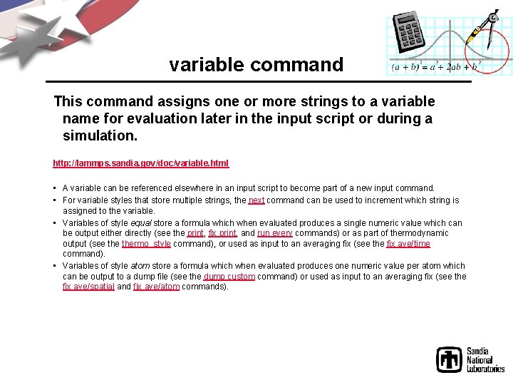
variable command This command assigns one or more strings to a variable name for evaluation later in the input script or during a simulation. http: //lammps. sandia. gov/doc/variable. html • A variable can be referenced elsewhere in an input script to become part of a new input command. • For variable styles that store multiple strings, the next command can be used to increment which string is assigned to the variable. • Variables of style equal store a formula which when evaluated produces a single numeric value which can be output either directly (see the print, fix print, and run every commands) or as part of thermodynamic output (see thermo_style command), or used as input to an averaging fix (see the fix ave/time command). • Variables of style atom store a formula which when evaluated produces one numeric value per atom which can be output to a dump file (see the dump custom command) or used as input to an averaging fix (see the fix ave/spatial and fix ave/atom commands).

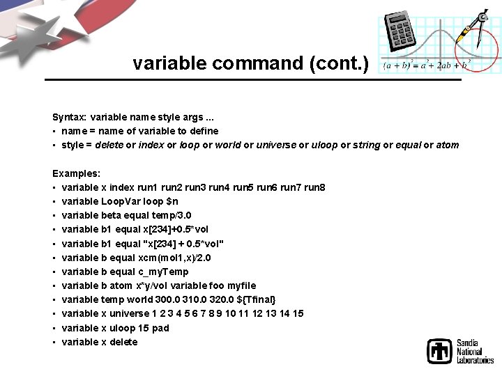
variable command (cont. ) Syntax: variable name style args. . . • name = name of variable to define • style = delete or index or loop or world or universe or uloop or string or equal or atom Examples: • variable x index run 1 run 2 run 3 run 4 run 5 run 6 run 7 run 8 • variable Loop. Var loop $n • variable beta equal temp/3. 0 • variable b 1 equal x[234]+0. 5*vol • variable b 1 equal "x[234] + 0. 5*vol" • variable b equal xcm(mol 1, x)/2. 0 • variable b equal c_my. Temp • variable b atom x*y/vol variable foo myfile • variable temp world 300. 0 310. 0 320. 0 ${Tfinal} • variable x universe 1 2 3 4 5 6 7 8 9 10 11 12 13 14 15 • variable x uloop 15 pad • variable x delete

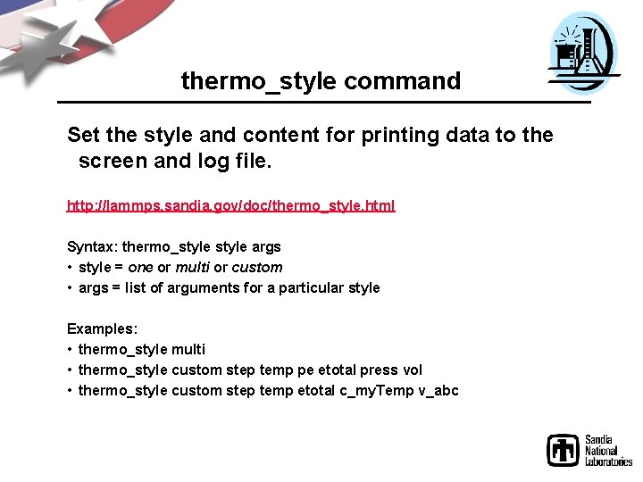
thermo_style command Set the style and content for printing data to the screen and log file. http: //lammps. sandia. gov/doc/thermo_style. html Syntax: thermo_style args • style = one or multi or custom • args = list of arguments for a particular style Examples: • thermo_style multi • thermo_style custom step temp pe etotal press vol • thermo_style custom step temp etotal c_my. Temp v_abc

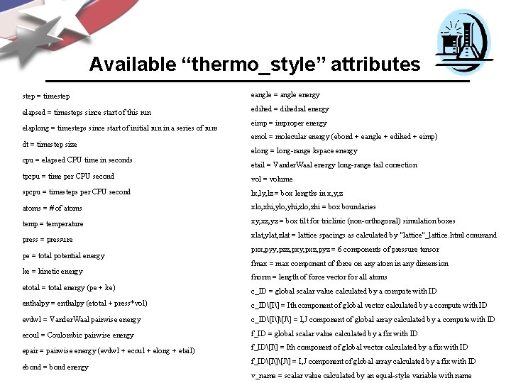
Available “thermo_style” attributes step = timestep eangle = angle energy elapsed = timesteps since start of this run edihed = dihedral energy elaplong = timesteps since start of initial run in a series of runs dt = timestep size cpu = elapsed CPU time in seconds eimp = improper energy emol = molecular energy (ebond + eangle + edihed + eimp) elong = long-range kspace energy etail = Vander. Waal energy long-range tail correction tpcpu = time per CPU second vol = volume spcpu = timesteps per CPU second lx, ly, lz = box lengths in x, y, z atoms = # of atoms xlo, xhi, ylo, yhi, zlo, zhi = box boundaries temp = temperature xy, xz, yz = box tilt for triclinic (non-orthogonal) simulation boxes press = pressure pe = total potential energy ke = kinetic energy etotal = total energy (pe + ke) xlat, ylat, zlat = lattice spacings as calculated by "lattice"_lattice. html command pxx, pyy, pzz, pxy, pxz, pyz = 6 components of pressure tensor fmax = max component of force on any atom in any dimension fnorm = length of force vector for all atoms c_ID = global scalar value calculated by a compute with ID enthalpy = enthalpy (etotal + press*vol) c_ID[I] = Ith component of global vector calculated by a compute with ID evdwl = Vander. Waal pairwise energy c_ID[I][J] = I, J component of global array calculated by a compute with ID ecoul = Coulombic pairwise energy f_ID = global scalar value calculated by a fix with ID epair = pairwise energy (evdwl + ecoul + elong + etail) f_ID[I] = Ith component of global vector calculated by a fix with ID ebond = bond energy f_ID[I][J] = I, J component of global array calculated by a fix with ID v_name = scalar value calculated by an equal-style variable with name

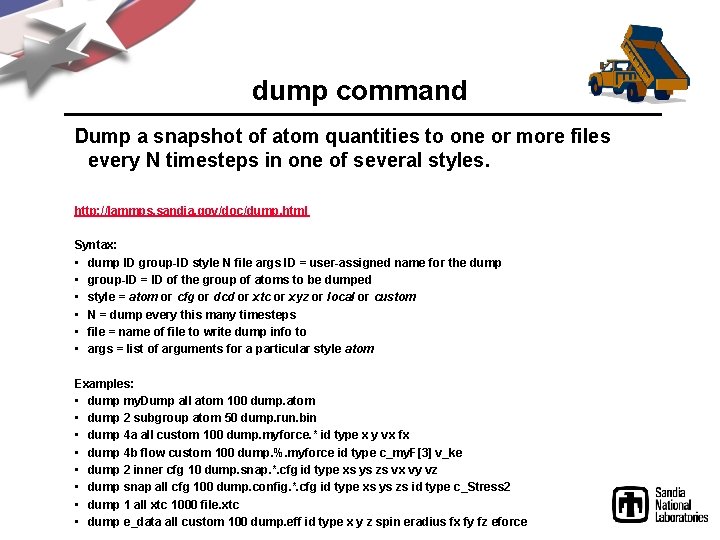
dump command Dump a snapshot of atom quantities to one or more files every N timesteps in one of several styles. http: //lammps. sandia. gov/doc/dump. html Syntax: • dump ID group-ID style N file args ID = user-assigned name for the dump • group-ID = ID of the group of atoms to be dumped • style = atom or cfg or dcd or xtc or xyz or local or custom • N = dump every this many timesteps • file = name of file to write dump info to • args = list of arguments for a particular style atom Examples: • dump my. Dump all atom 100 dump. atom • dump 2 subgroup atom 50 dump. run. bin • dump 4 a all custom 100 dump. myforce. * id type x y vx fx • dump 4 b flow custom 100 dump. %. myforce id type c_my. F[3] v_ke • dump 2 inner cfg 10 dump. snap. *. cfg id type xs ys zs vx vy vz • dump snap all cfg 100 dump. config. *. cfg id type xs ys zs id type c_Stress 2 • dump 1 all xtc 1000 file. xtc • dump e_data all custom 100 dump. eff id type x y z spin eradius fx fy fz eforce

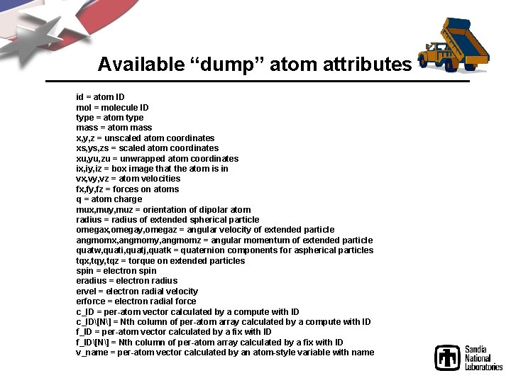
Available “dump” atom attributes id = atom ID mol = molecule ID type = atom type mass = atom mass x, y, z = unscaled atom coordinates xs, ys, zs = scaled atom coordinates xu, yu, zu = unwrapped atom coordinates ix, iy, iz = box image that the atom is in vx, vy, vz = atom velocities fx, fy, fz = forces on atoms q = atom charge mux, muy, muz = orientation of dipolar atom radius = radius of extended spherical particle omegax, omegay, omegaz = angular velocity of extended particle angmomx, angmomy, angmomz = angular momentum of extended particle quatw, quati, quatj, quatk = quaternion components for aspherical particles tqx, tqy, tqz = torque on extended particles spin = electron spin eradius = electron radius ervel = electron radial velocity erforce = electron radial force c_ID = per-atom vector calculated by a compute with ID c_ID[N] = Nth column of per-atom array calculated by a compute with ID f_ID = per-atom vector calculated by a fix with ID f_ID[N] = Nth column of per-atom array calculated by a fix with ID v_name = per-atom vector calculated by an atom-style variable with name

Live demo #3 1. Modify the LAMMPS input script from demo #2 so that it includes at least one example of each of the following six commands: 1. 2. 3. 4. 5. 6. fix compute pair_style variable thermo_style dump 2. Run LAMMPS with the modified input script.

Discussion outline 1. 2. 3. 4. 5. 6. 7. 8. 9. 10. 11. MD basics Why use LAMMPS? Live demo #1 Basic information about LAMMPS Live demo #2 Six very useful LAMMPS commands Live demo #3 Vignettes of some LAMMPS research Future areas of LAMMPS development How to add a new feature to LAMMPS Homework assignment

Vignettes of some LAMMPS research • • • Interfaces in melting solids Adhesion properties of polymers Shear response in metals Tensile pull on nanowires Surface growth on mismatched lattice Shock-induced phase transformations Silica nanopores for water desalination Coated nanoparticles in solution and at interfaces Self-assembly (2 d micelles and 3 d lipid bilayers) Rhodopsin protein isomerization Whole vesicle simulation Radiation damage

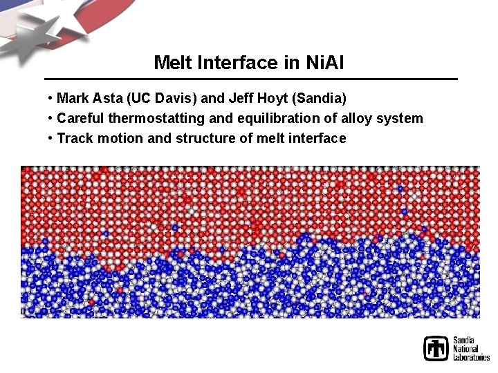
Melt Interface in Ni. Al • Mark Asta (UC Davis) and Jeff Hoyt (Sandia) • Careful thermostatting and equilibration of alloy system • Track motion and structure of melt interface

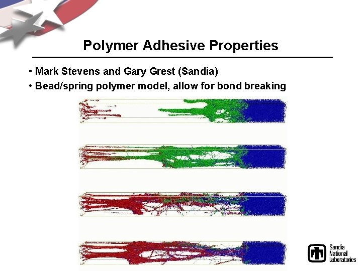
Polymer Adhesive Properties • Mark Stevens and Gary Grest (Sandia) • Bead/spring polymer model, allow for bond breaking

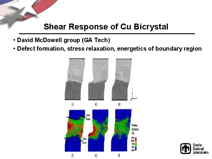
Shear Response of Cu Bicrystal • David Mc. Dowell group (GA Tech) • Defect formation, stress relaxation, energetics of boundary region

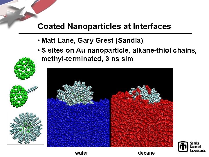
Coated Nanoparticles at Interfaces • Matt Lane, Gary Grest (Sandia) • S sites on Au nanoparticle, alkane-thiol chains, methyl-terminated, 3 ns sim water decane

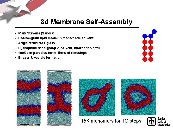
3 d Membrane Self-Assembly • • • Mark Stevens (Sandia) Coarse-grain lipid model in monomeric solvent Angle terms for rigidity Hydrophilic head-group & solvent, hydrophobic tail 100 Ks of particles for millions of timesteps Bilayer & vesicle formation 15 K monomers for 1 M steps

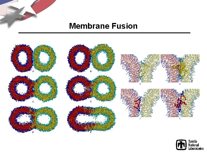
Membrane Fusion • Gently push together. . .

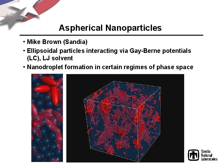
Aspherical Nanoparticles • Mike Brown (Sandia) • Ellipsoidal particles interacting via Gay-Berne potentials (LC), LJ solvent • Nanodroplet formation in certain regimes of phase space

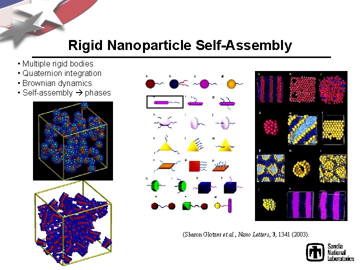
Rigid Nanoparticle Self-Assembly • Multiple rigid bodies • Quaternion integration • Brownian dynamics • Self-assembly phases (Sharon Glotzer et al. , Nano Letters, 3, 1341 (2003).

LAMMPS’s Reactive Force Fields Capability Why Reactive Force Fields? • Material behavior often dominated by chemical processes • HE, Complex Solids, Polymer Aging • Quantum methods limited to hundreds of atoms • Ordinary classical force fields limited accuracy • We need to have the best of both worlds Reactive force fields Why build Reactive Force Fields into LAMMPS? • Reactive force fields typically exist as custom serial MD codes • LAMMPS is a general parallel MD code

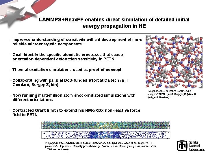
LAMMPS+Reax. FF enables direct simulation of detailed initial energy propagation in HE – Improved understanding of sensitivity will aid development of more reliable microenergetic components – Goal: Identify the specific atomistic processes that cause orientation-dependent detonation sensitivity in PETN – Thermal excitation simulations used as proof-of-concept – Collaborating with parallel Do. D-funded effort at Caltech (Bill Goddard, Sergey Zybin) – Now running multi-million atom shock-initiated simulations with different orientations Complex molecular structure of unreacted tetragonal PETN crystal, C (gray), N (blue), O (red), and H (white). – Contracted Grant Smith to extend his HMX/RDX non-reactive force field to PETN Propagation of reaction front due to thermal excitation of a thin layer at the center of the sample for 10 picoseconds. Top: atoms colored by potential energy. Bottom: atoms colored by temperature (atoms below 1000 K are not shown).

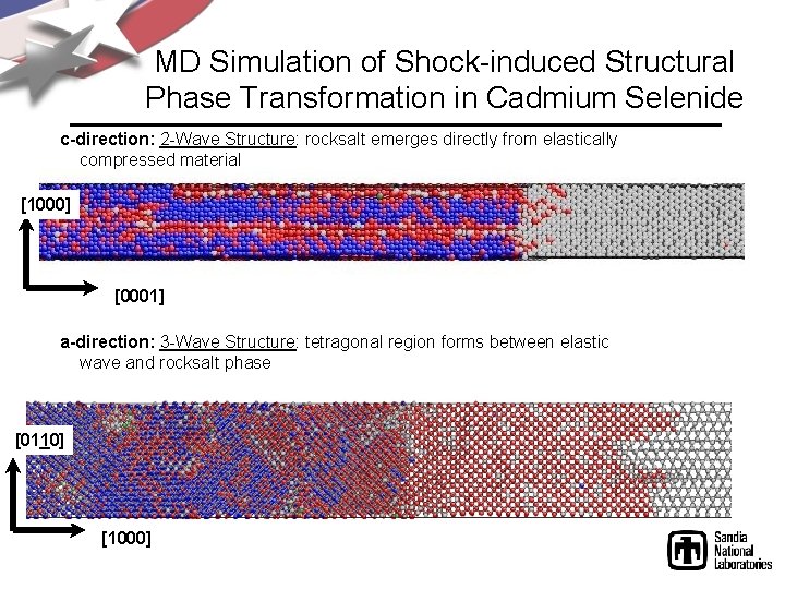
MD Simulation of Shock-induced Structural Phase Transformation in Cadmium Selenide c-direction: 2 -Wave Structure: rocksalt emerges directly from elastically compressed material [1000] [0001] a-direction: 3 -Wave Structure: tetragonal region forms between elastic wave and rocksalt phase [0110] [1000]

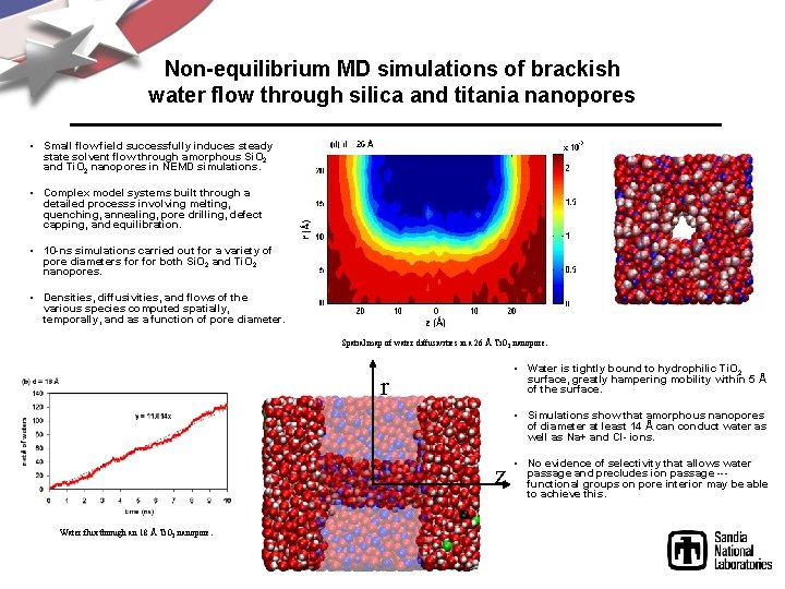
Non-equilibrium MD simulations of brackish water flow through silica and titania nanopores • Small flow field successfully induces steady state solvent flow through amorphous Si. O 2 and Ti. O 2 nanopores in NEMD simulations. • Complex model systems built through a detailed processs involving melting, quenching, annealing, pore drilling, defect capping, and equilibration. • 10 -ns simulations carried out for a variety of pore diameters for both Si. O 2 and Ti. O 2 nanopores. • Densities, diffusivities, and flows of the various species computed spatially, temporally, and as a function of pore diameter. Spatial map of water diffusivities in a 26 Å Ti. O 2 nanopore. • Water is tightly bound to hydrophilic Ti. O 2 surface, greatly hampering mobility within 5 Å of the surface. r • Simulations show that amorphous nanopores of diameter at least 14 Å can conduct water as well as Na+ and Cl- ions. z Water flux through an 18 Å Ti. O 2 nanopore. • No evidence of selectivity that allows water passage and precludes ion passage --- functional groups on pore interior may be able to achieve this.

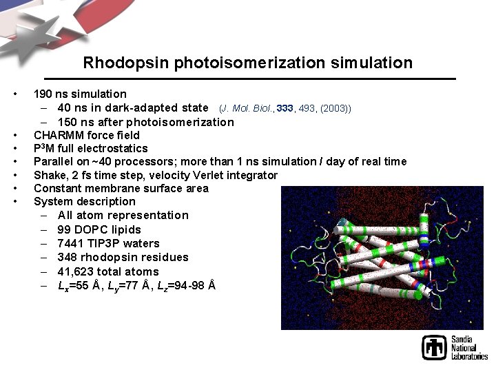
Rhodopsin photoisomerization simulation • 190 ns simulation – 40 ns in dark-adapted state (J. Mol. Biol. , 333, 493, (2003)) – 150 ns after photoisomerization • • • CHARMM force field P 3 M full electrostatics Parallel on ~40 processors; more than 1 ns simulation / day of real time Shake, 2 fs time step, velocity Verlet integrator Constant membrane surface area System description – – – All atom representation 99 DOPC lipids 7441 TIP 3 P waters 348 rhodopsin residues 41, 623 total atoms Lx=55 Å, Ly=77 Å, Lz=94 -98 Å

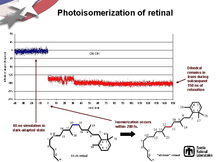
Photoisomerization of retinal Dihedral remains in trans during subsequent 150 ns of relaxation 40 -ns simulation in dark-adapted state Isomerization occurs within 200 fs.

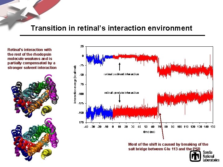
Transition in retinal’s interaction environment Retinal’s interaction with the rest of the rhodopsin molecule weakens and is partially compensated by a stronger solvent interaction Most of the shift is caused by breaking of the salt bridge between Glu 113 and the PSB

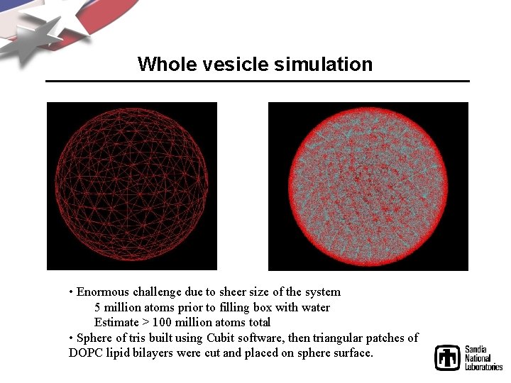
Whole vesicle simulation • Enormous challenge due to sheer size of the system 5 million atoms prior to filling box with water Estimate > 100 million atoms total • Sphere of tris built using Cubit software, then triangular patches of DOPC lipid bilayers were cut and placed on sphere surface.

Radiation damage simulations ► Radiation damage is directly relevant to several nuclear energy applications § § § Reactor core materials Fuels and cladding Waste forms ► Experiments are not able to elucidate the mechanism involved in structural disorder following irradiation ► Classical simulations can help provide atomistic detail for relaxation processes involved ► Electronic effects have been successfully used in cascade simulations of metallic systems

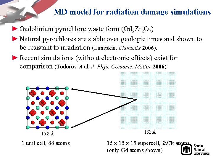
MD model for radiation damage simulations ► Gadolinium pyrochlore waste form (Gd 2 Zr 2 O 7) ► Natural pyrochlores are stable over geologic times and shown to be resistant to irradiation (Lumpkin, Elements 2006). ► Recent simulations (without electronic effects) exist for comparison (Todorov et al, J. Phys. Condens. Matter 2006). 10. 8 Å 1 unit cell, 88 atoms 162 Å 15 x 15 supercell, 297 k atoms (only Gd atoms shown)

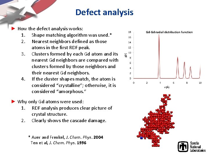
Defect analysis ► How the defect analysis works: 1. Shape matching algorithm was used. * 2. Nearest neighbors defined as those atoms in the first RDF peak. 3. Clusters formed by each Gd atom and its nearest Gd neighbors are compared with clusters formed by those neighbors and their nearest Gd neighbors. 4. If the cluster shapes match, the atom is considered “crystalline”; otherwise, it is considered “amorphous. ” ► Why only Gd atoms were used: 1. RDF analysis produces clear picture of crystal structure. 2. Clearly shows the cascade damage. * Auer and Frenkel, J. Chem. Phys. 2004 Ten et al, J. Chem. Phys. 1996

Discussion outline 1. 2. 3. 4. 5. 6. 7. 8. 9. 10. 11. MD basics Why use LAMMPS? Live demo #1 Basic information about LAMMPS Live demo #2 Six very useful LAMMPS commands Live demo #3 Vignettes of some LAMMPS research Future areas of LAMMPS development How to add a new feature to LAMMPS Homework assignment

Future areas of LAMMPS development • Alleviations of time-scale and spatial-scale limitations • Improved force fields for better molecular physics • New features for the convenience of users

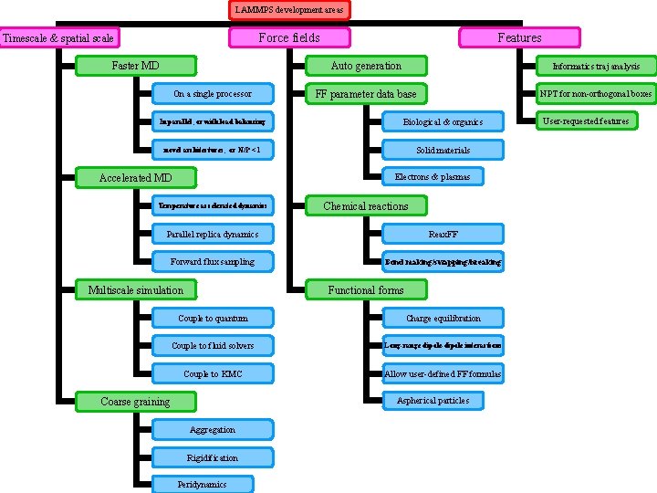
LAMMPS development areas Force fields Timescale & spatial scale Faster MD On a single processor Features Auto generation Informatics traj analysis FF parameter data base NPT for non-orthogonal boxes In parallel, or with load balancing Biological & organics novel architectures, or N/P < 1 Solid materials Electrons & plasmas Accelerated MD Temperature accelerated dynamics Chemical reactions Parallel replica dynamics Reax. FF Forward flux sampling Bond making/swapping/breaking Functional forms Multiscale simulation Couple to quantum Charge equilibration Couple to fluid solvers Long-range dipole-dipole interactions Couple to KMC Allow user-defined FF formulas Aspherical particles Coarse graining Aggregation Rigidification Peridynamics User-requested features

How to add a new feature to LAMMPS Case study: simulation of gas uptake into microporous materials.

What are microporous materials and what are their uses? “A microporous material is a material containing pores with diameters less than 2 nm. Porous materials are classified into several kinds by their size. ” “Microporous materials have pore diameters of less than 2 nm, mesoporous materials have pore diameters between 2 nm and 50 nm and macroporous materials have pore diameters of greater than 50 nm. ” • Facilitate contaminant-free exchange of gases. Mold spores, bacteria, and other airborne contaminants will become trapped, while allowing gases to pass through the material. • Microporous materials are also used in first aid. http: //en. wikipedia. org/wiki/Microporous_material • Radioactive materials separation or storage.

What are ZIFs? ZIF = zeolitic imidazolate framework “ZIFs are one kind of metal-organic frameworks' subsidiaries which could be used to keep industrial emissions of carbon dioxide out of the atmosphere. One litre of the crystals could store about 83 litres of CO 2. The crystals are non-toxic and require little energy to create, making them an attractive possibility for carbon capture and storage. The porous structures can be heated to high temperatures without decomposing and can be boiled in water or solvents for a week and remain stable, making them suitable for use in hot, energy-producing environments like power plants. ” “Like zeolites and other porous materials, zeolitic imidazolate framework membranes can be used for the separation of gases because of its highly porous structure, large accessible pore volume with fully exposed edges and faces of the organic links, pore apertures in the range of the kinetic diameter of several gas molecules, and high CO 2 adsorption capacity. ” http: //en. wikipedia. org/wiki/Zeolitic_imidazolate_frameworks

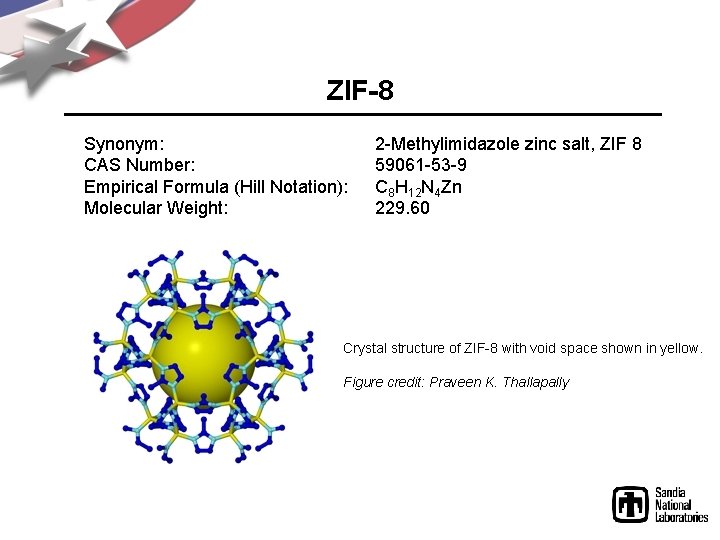
ZIF-8 Synonym: CAS Number: Empirical Formula (Hill Notation): Molecular Weight: 2 -Methylimidazole zinc salt, ZIF 8 59061 -53 -9 C 8 H 12 N 4 Zn 229. 60 Crystal structure of ZIF-8 with void space shown in yellow. Figure credit: Praveen K. Thallapally

What questions about iodine uptake in ZIF-8 might we hope to address with molecular simulation? 1. How much I 2 can ZIF-8 hold? (What is the loading vs pressure relationship? Can we compute a loading iostherm? ) 2. How mobile is I 2 once it is adsorbed within the ZIF-8 framework? 3. What is the structure of I 2 -loaded ZIF-8 and where are the main binding locations? 4. How well do simulation results compare with available experimental measurements?

What simulation tools might we use to address our questions? Molecular dynamics (MD): is computer simulation of physical movements by atoms and molecules. http: //en. wikipedia. org/wiki/Molecular_dynamics Monte Carlo (MC): This approach relies on statistical mechanics rather than molecular dynamics. Instead of trying to reproduce the dynamics of a system, it generates states according to appropriate Boltzmann probabilities. (http: //en. wikipedia. org/wiki/Monte_Carlo_molecular_modeling) Grand canonical Monte Carlo (GCMC): a very versatile and powerful Monte Carlo technique that explicitly accounts for density fluctuations at fixed volume and temperature. This is achieved by means of trial insertion and deletion of molecules. Although this feature has made it the preferred choice for the study of interfacial phenomena, in the last decade grandcanonical ensemble simulations have also found widespread applications in the study of bulk properties. Such applications had been hitherto limited by the very low particle insertion and deletion probabilities, but the development of the configurational bias grand canonical technique has very much improved the situation. (http: //www. sklogwiki. org) Gibbs ensemble Monte Carlo (GEMC): The Gibbs ensemble Monte Carlo method has been specifically designed to characterize phase transitions. It was mainly developed by Panagiotopoulos (Refs. 1 and 2) to avoid the problem of finite size interfacial effects. In this method, an NVT (or Np. T) ensemble containing two (or more) species is divided into two (or more) boxes. In addition to the usual particle moves in each one of the boxes, the algorithm includes moves steps to change the volume and composition of the boxes at mechanical and chemical equilibrium. Transferring a chain molecule from a box to the other requires the use of an efficient method to insert chains. The configurational bias method is specially recommended for this purpose. (http: //www. sklogwiki. org)

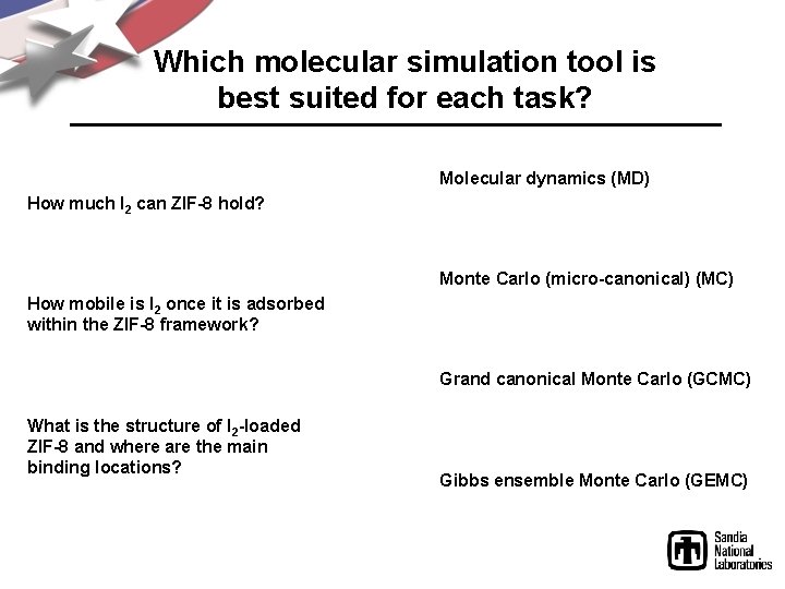
Which molecular simulation tool is best suited for each task? Molecular dynamics (MD) How much I 2 can ZIF-8 hold? Monte Carlo (micro-canonical) (MC) How mobile is I 2 once it is adsorbed within the ZIF-8 framework? Grand canonical Monte Carlo (GCMC) What is the structure of I 2 -loaded ZIF-8 and where are the main binding locations? Gibbs ensemble Monte Carlo (GEMC)

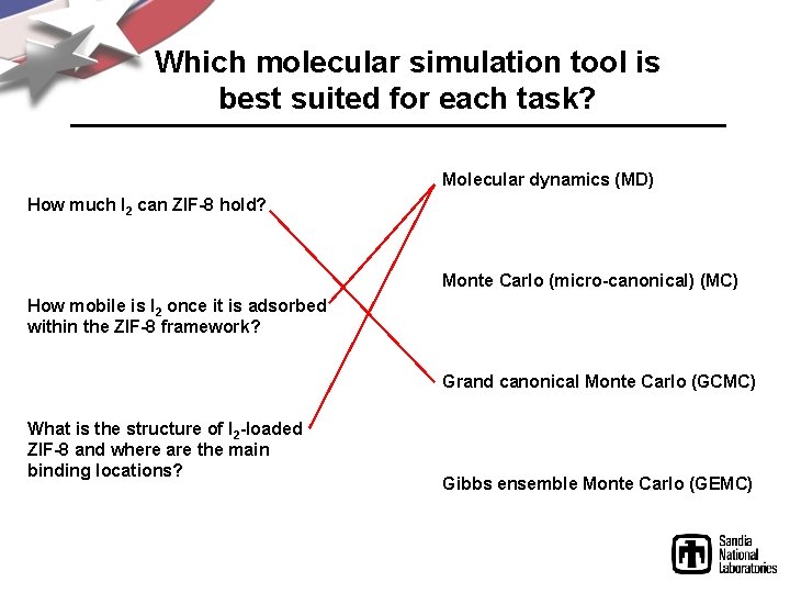
Which molecular simulation tool is best suited for each task? Molecular dynamics (MD) How much I 2 can ZIF-8 hold? Monte Carlo (micro-canonical) (MC) How mobile is I 2 once it is adsorbed within the ZIF-8 framework? Grand canonical Monte Carlo (GCMC) What is the structure of I 2 -loaded ZIF-8 and where are the main binding locations? Gibbs ensemble Monte Carlo (GEMC)

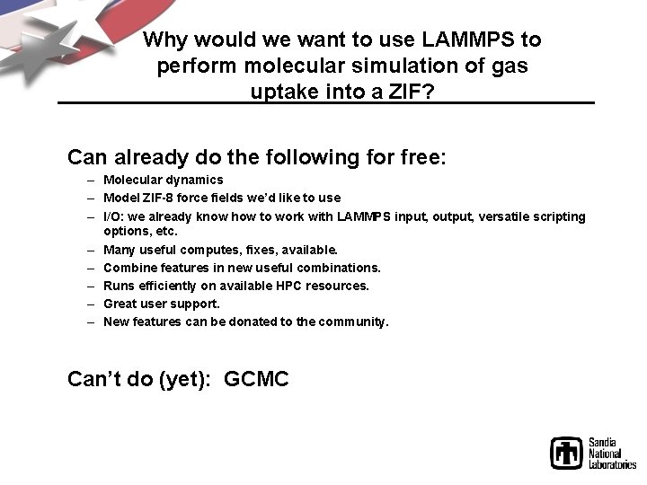
Why would we want to use LAMMPS to perform molecular simulation of gas uptake into a ZIF? Can already do the following for free: – Molecular dynamics – Model ZIF-8 force fields we’d like to use – I/O: we already know how to work with LAMMPS input, output, versatile scripting options, etc. – Many useful computes, fixes, available. – Combine features in new useful combinations. – Runs efficiently on available HPC resources. – Great user support. – New features can be donated to the community. Can’t do (yet): GCMC

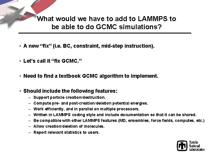
What would we have to add to LAMMPS to be able to do GCMC simulations? • A new “fix” (i. e. BC, constraint, mid-step instruction). • Let’s call it “fix GCMC. ” • Need to find a textbook GCMC algorithm to implement. • Should include the following features: – – – – Support particle creation/destruction. Compute pre- and post-creation/deletion potential energies. Work efficiently, and in parallel on multiple processors. Written in LAMMPS coding style and include documentation so that it can be shared. Be compatible with other LAMMPS features (MD, ensembles, force fields, computes, etc. ) Allow creation/deletion of molecules. Report relevant statistics to users.

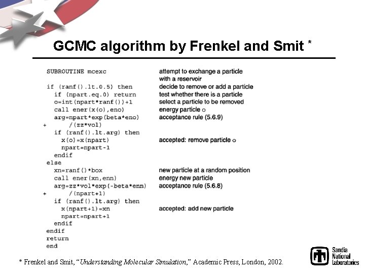
GCMC algorithm by Frenkel and Smit * * Frenkel and Smit, “Understanding Molecular Simulation, ” Academic Press, London, 2002.

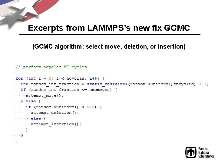
Excerpts from LAMMPS’s new fix GCMC (GCMC algorithm: select move, deletion, or insertion)

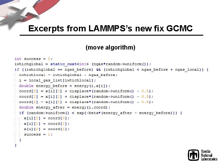
Excerpts from LAMMPS’s new fix GCMC (move algorithm)

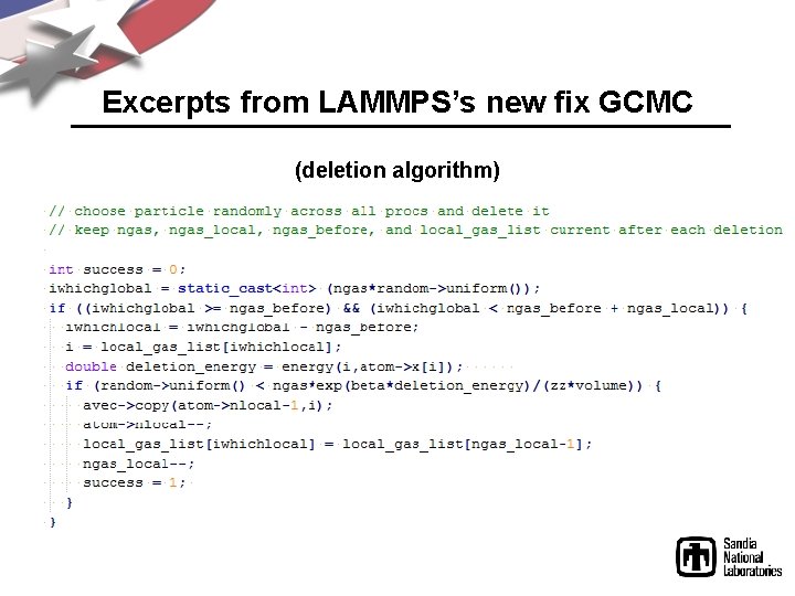
Excerpts from LAMMPS’s new fix GCMC (deletion algorithm)

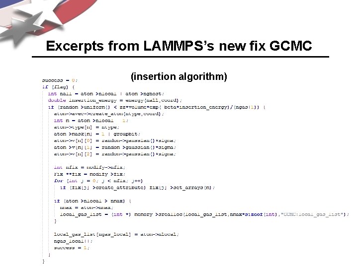
Excerpts from LAMMPS’s new fix GCMC (insertion algorithm)

How do we know that we’ve implemented the algorithm correctly? Verification exercise: code-to-code comparison versus an established Monte Carlo code (Towhee). Gas = Kr (with LJ parameters from Pellenq and Levitz) T = 300 K m = -10. 284 kcal/mol P = ? If ideal gas: üP(ideal gas) = 1 bar üAlso, from Towhee calculation: P(Towhee) = 1 bar üCorrected a sign error in the new code that caused a slight discrepancy üNow, with our new fix GCMC for LAMMPS, we have: P(LAMMPS) = 1 bar

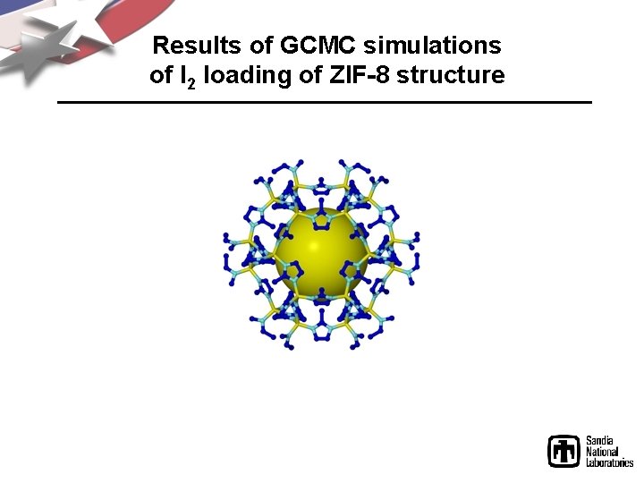
Results of GCMC simulations of I 2 loading of ZIF-8 structure

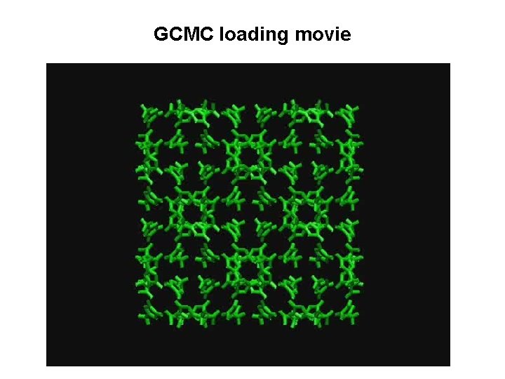
GCMC loading movie

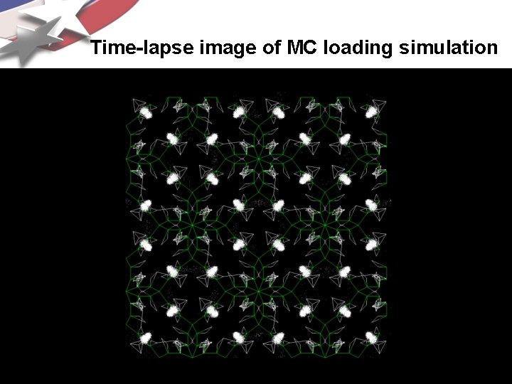
Time-lapse image of MC loading simulation

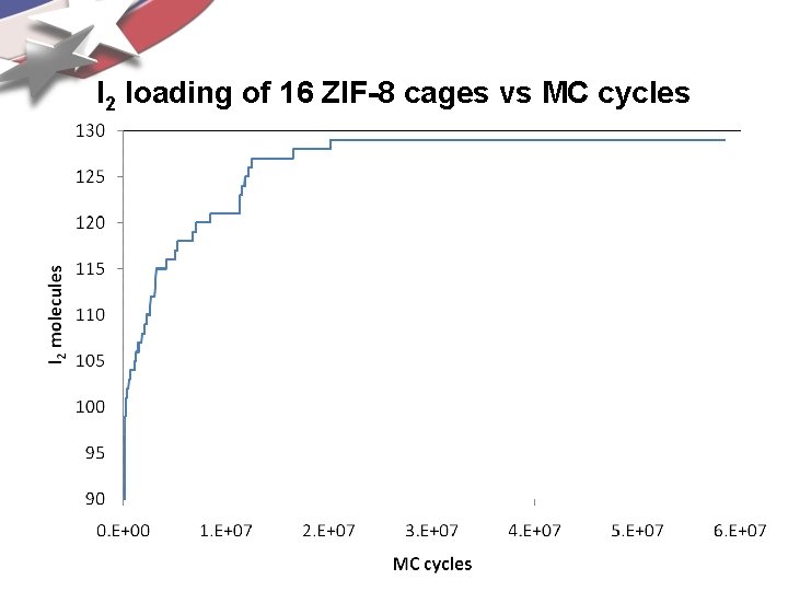
I 2 loading of 16 ZIF-8 cages vs MC cycles

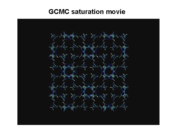
GCMC saturation movie

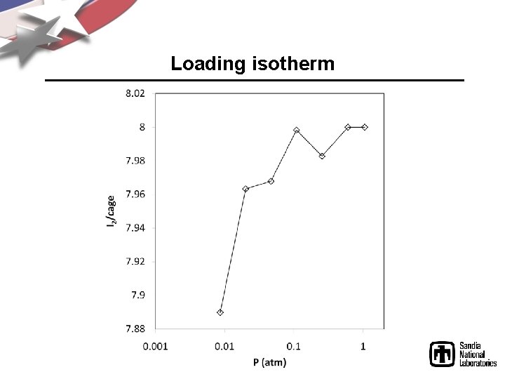
Loading isotherm

Homework assignment Repeat the live demo exercises yourself, with your own personal modifications.

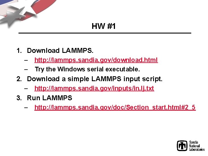
HW #1 1. Download LAMMPS. – – http: //lammps. sandia. gov/download. html Try the Windows serial executable. 2. Download a simple LAMMPS input script. – http: //lammps. sandia. gov/inputs/in. lj. txt 3. Run LAMMPS – http: //lammps. sandia. gov/doc/Section_start. html#2_5

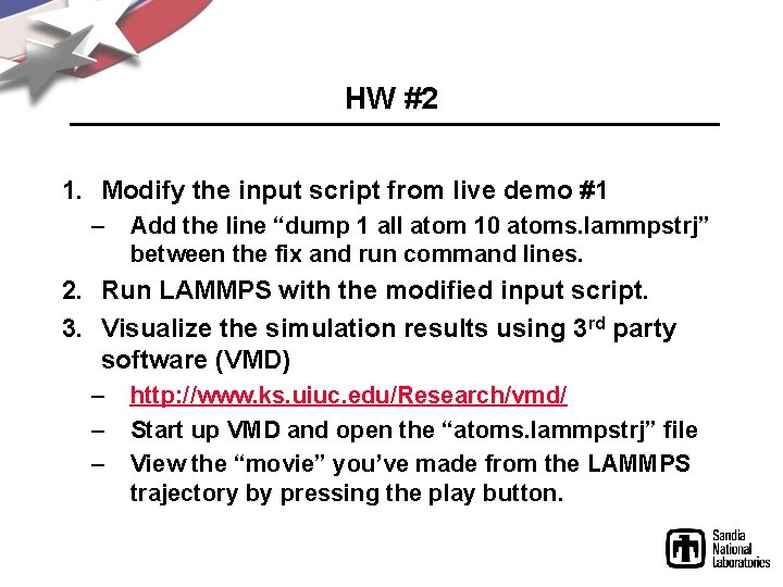
HW #2 1. Modify the input script from live demo #1 – Add the line “dump 1 all atom 10 atoms. lammpstrj” between the fix and run command lines. 2. Run LAMMPS with the modified input script. 3. Visualize the simulation results using 3 rd party software (VMD) – – – http: //www. ks. uiuc. edu/Research/vmd/ Start up VMD and open the “atoms. lammpstrj” file View the “movie” you’ve made from the LAMMPS trajectory by pressing the play button.

HW #3 1. Modify the LAMMPS input script from demo #2 so that it includes at least one example of each of the following six commands: 1. 2. 3. 4. 5. 6. fix compute pair_style variable thermo_style dump 2. Run LAMMPS with the modified input script.