A brief overview of the classical linear regression

A brief overview of the classical linear regression model(continued) SHAHROOD UNIVERSITY OF TECHNOLOGY 1

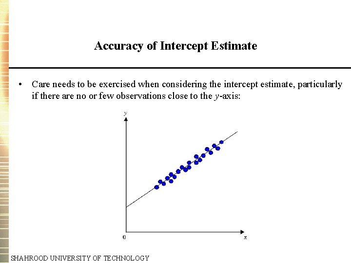
Accuracy of Intercept Estimate • Care needs to be exercised when considering the intercept estimate, particularly if there are no or few observations close to the y-axis: SHAHROOD UNIVERSITY OF TECHNOLOGY

The Population and the Sample • The population is the total collection of all objects or people to be studied, for example, • Interested in predicting outcome of an election Population of interest the entire electorate • A sample is a selection of just some items from the population. • A random sample is a sample in which each individual item in the population is equally likely to be drawn. SHAHROOD UNIVERSITY OF TECHNOLOGY

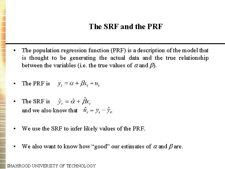
The SRF and the PRF • The population regression function (PRF) is a description of the model that is thought to be generating the actual data and the true relationship between the variables (i. e. the true values of and ). • The PRF is • The SRF is and we also know that . • We use the SRF to infer likely values of the PRF. • We also want to know how “good” our estimates of and are. SHAHROOD UNIVERSITY OF TECHNOLOGY

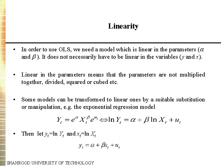
Linearity • In order to use OLS, we need a model which is linear in the parameters ( and ). It does not necessarily have to be linear in the variables (y and x). • Linear in the parameters means that the parameters are not multiplied together, divided, squared or cubed etc. • Some models can be transformed to linear ones by a suitable substitution or manipulation, e. g. the exponential regression model • Then let yt=ln Yt and xt=ln Xt SHAHROOD UNIVERSITY OF TECHNOLOGY

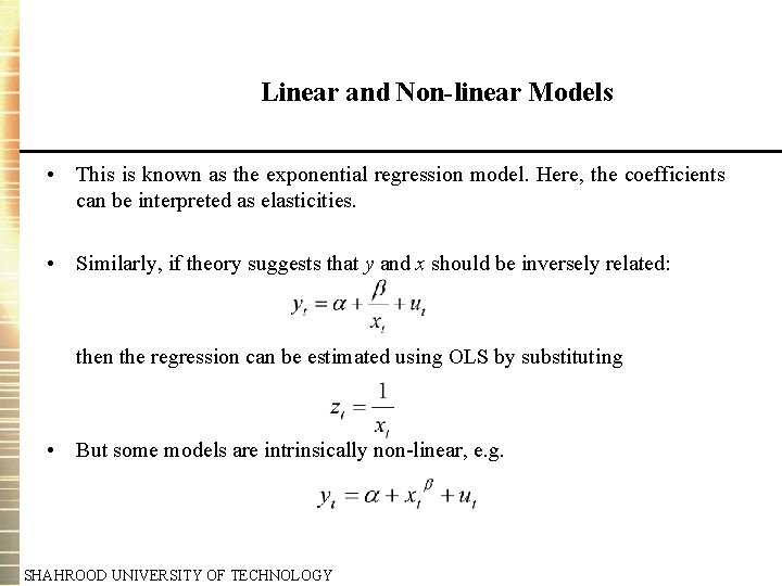
Linear and Non-linear Models • This is known as the exponential regression model. Here, the coefficients can be interpreted as elasticities. • Similarly, if theory suggests that y and x should be inversely related: then the regression can be estimated using OLS by substituting • But some models are intrinsically non-linear, e. g. SHAHROOD UNIVERSITY OF TECHNOLOGY

Estimator or Estimate? • Estimators are the formulae used to calculate the coefficients • Estimates are the actual numerical values for the coefficients. SHAHROOD UNIVERSITY OF TECHNOLOGY

The Assumptions Underlying the Classical Linear Regression Model (CLRM) • The model which we have used is known as the classical linear regression model. • We observe data for xt, but since yt also depends on ut, we must be specific about how the ut are generated. • We usually make the following set of assumptions about the ut’s (the unobservable error terms): • Technical Notation Interpretation 1. E(ut) = 0 The errors have zero mean 2. Var (ut) = 2 The variance of the errors is constant and finite over all values of xt 3. Cov (ui, uj)=0 The errors are statistically independent of one another 4. Cov (ut, xt)=0 No relationship between the error and corresponding x variate SHAHROOD UNIVERSITY OF TECHNOLOGY

The Assumptions Underlying the CLRM Again • An alternative assumption to 4. , which is slightly stronger, is that the xt’s are non-stochastic or fixed in repeated samples. • A fifth assumption is required if we want to make inferences about the population parameters (the actual and ) from the sample parameters ( and ) • Additional Assumption 5. ut is normally distributed SHAHROOD UNIVERSITY OF TECHNOLOGY

Properties of the OLS Estimator • If assumptions 1. through 4. hold, then the estimators and determined by OLS are known as Best Linear Unbiased Estimators (BLUE). What does the acronym stand for? • “Estimator” • “Linear” • “Unbiased” • “Best” - is an estimator of the true value of . - is a linear estimator - On average, the actual value of the and ’s will be equal to the true values. - means that the OLS estimator has minimum variance among the class of linear unbiased estimators. The Gauss-Markov theorem proves that the OLS estimator is best. SHAHROOD UNIVERSITY OF TECHNOLOGY

Consistency/Unbiasedness/Efficiency • Consistent The least squares estimators and are consistent. That is, the estimates will converge to their true values as the sample size increases to infinity. Need the assumptions E(xtut)=0 and Var(ut)= 2 < to prove this. Consistency implies that • Unbiased The least squares estimates of and are unbiased. That is E( )= and E( )= Thus on average the estimated value will be equal to the true values. To prove this also requires the assumption that E(ut)=0. Unbiasedness is a stronger condition than consistency. • Efficiency An estimator of parameter is said to be efficient if it is unbiased and no other unbiased estimator has a smaller variance. If the estimator is efficient, we are minimising the probability that it is a long way off from the true value of . SHAHROOD UNIVERSITY OF TECHNOLOGY