A brief overview of the classical linear regression

A brief overview of the classical linear regression model(cont) SHAHROOD UNIVERSITY OF TECH

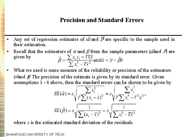
Precision and Standard Errors • Any set of regression estimates of and are specific to the sample used in their estimation. • Recall that the estimators of and from the sample parameters ( and ) are given by • What we need is some measure of the reliability or precision of the estimators ( and ). The precision of the estimate is given by its standard error. Given assumptions 1 - 4 above, then the standard errors can be shown to be given by where s is the estimated standard deviation of the residuals. SHAHROOD UNIVERSITY OF TECH

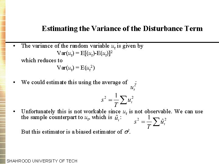
Estimating the Variance of the Disturbance Term • The variance of the random variable ut is given by Var(ut) = E[(ut)-E(ut)]2 which reduces to Var(ut) = E(ut 2) • We could estimate this using the average of : • Unfortunately this is not workable since ut is not observable. We can use the sample counterpart to ut, which is : But this estimator is a biased estimator of 2. SHAHROOD UNIVERSITY OF TECH

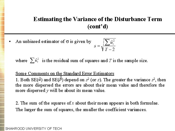
Estimating the Variance of the Disturbance Term (cont’d) • An unbiased estimator of is given by where is the residual sum of squares and T is the sample size. Some Comments on the Standard Error Estimators 1. Both SE( ) and SE( ) depend on s 2 (or s). The greater the variance s 2, then the more dispersed the errors are about their mean value and therefore the more dispersed y will be about its mean value. 2. The sum of the squares of x about their mean appears in both formulae. The larger the sum of squares, the smaller the coefficient variances. SHAHROOD UNIVERSITY OF TECH

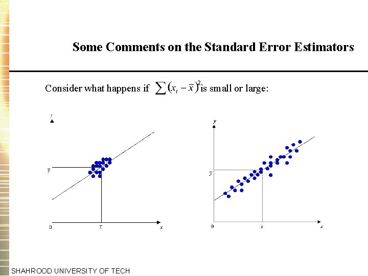
Some Comments on the Standard Error Estimators Consider what happens if SHAHROOD UNIVERSITY OF TECH is small or large:

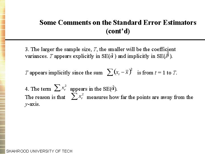
Some Comments on the Standard Error Estimators (cont’d) 3. The larger the sample size, T, the smaller will be the coefficient variances. T appears explicitly in SE( ) and implicitly in SE( ). T appears implicitly since the sum is from t = 1 to T. 4. The term appears in the SE( ). The reason is that measures how far the points are away from the y-axis. SHAHROOD UNIVERSITY OF TECH

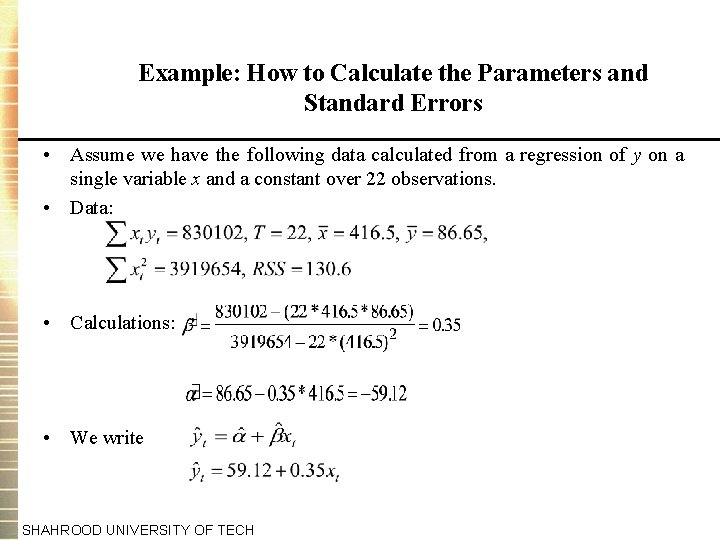
Example: How to Calculate the Parameters and Standard Errors • Assume we have the following data calculated from a regression of y on a single variable x and a constant over 22 observations. • Data: • Calculations: • We write SHAHROOD UNIVERSITY OF TECH

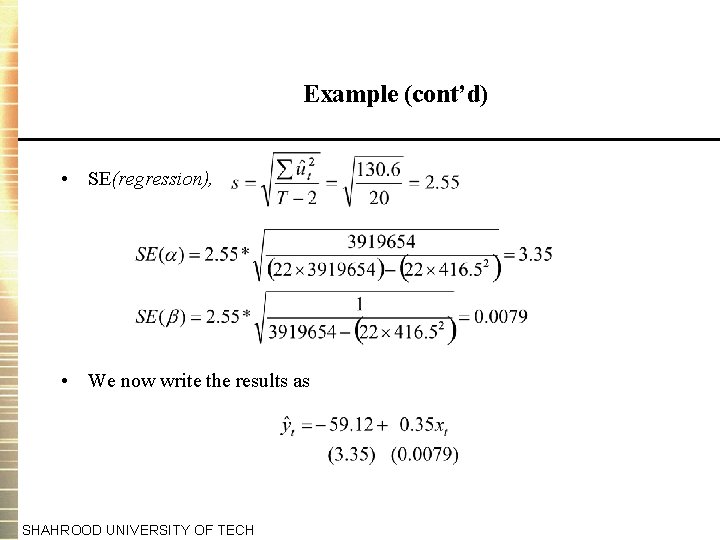
Example (cont’d) • SE(regression), • We now write the results as SHAHROOD UNIVERSITY OF TECH

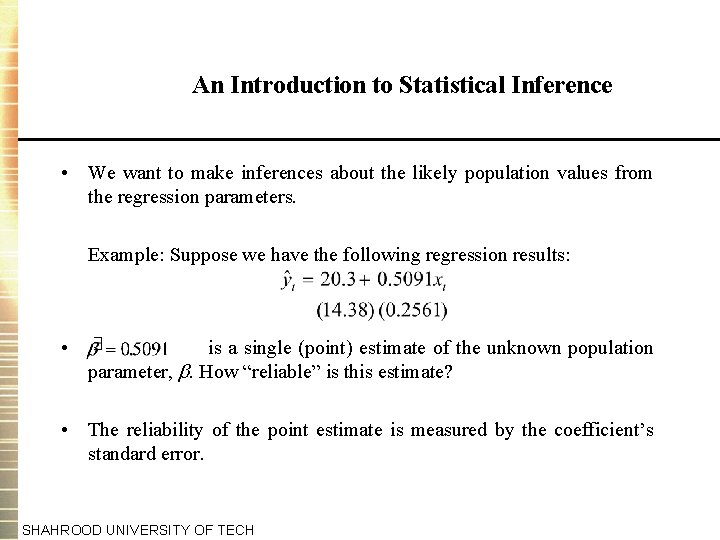
An Introduction to Statistical Inference • We want to make inferences about the likely population values from the regression parameters. Example: Suppose we have the following regression results: • is a single (point) estimate of the unknown population parameter, . How “reliable” is this estimate? • The reliability of the point estimate is measured by the coefficient’s standard error. SHAHROOD UNIVERSITY OF TECH

Hypothesis Testing: Some Concepts • We can use the information in the sample to make inferences about the population. • We will always have two hypotheses that go together, the null hypothesis (denoted H 0) and the alternative hypothesis (denoted H 1). • The null hypothesis is the statement or the statistical hypothesis that is actually being tested. The alternative hypothesis represents the remaining outcomes of interest. • For example, suppose given the regression results above, we are interested in the hypothesis that the true value of is in fact 0. 5. We would use the notation H 0 : = 0. 5 H 1 : 0. 5 This would be known as a two sided test. SHAHROOD UNIVERSITY OF TECH

One-Sided Hypothesis Tests • Sometimes we may have some prior information that, for example, we would expect > 0. 5 rather than < 0. 5. In this case, we would do a one-sided test: H 0 : = 0. 5 H 1 : > 0. 5 or we could have had H 0 : = 0. 5 H 1 : < 0. 5 • There are two ways to conduct a hypothesis test: via the test of significance approach or via the confidence interval approach. SHAHROOD UNIVERSITY OF TECH

The Probability Distribution of the Least Squares Estimators • We assume that ut N(0, 2) • Since the least squares estimators are linear combinations of the random variables i. e. • The weighted sum of normal random variables is also normally distributed, so N( , Var( )) • What if the errors are not normally distributed? Will the parameter estimates still be normally distributed? • Yes, if the other assumptions of the CLRM hold, and the sample size is sufficiently large. SHAHROOD UNIVERSITY OF TECH

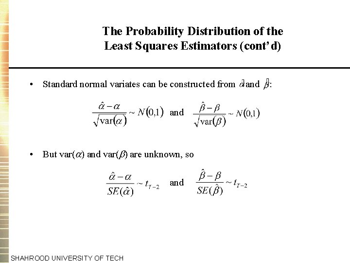
The Probability Distribution of the Least Squares Estimators (cont’d) • Standard normal variates can be constructed from and : and • But var( ) and var( ) are unknown, so and SHAHROOD UNIVERSITY OF TECH

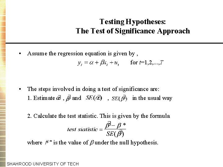
Testing Hypotheses: The Test of Significance Approach • Assume the regression equation is given by , for t=1, 2, . . . , T • The steps involved in doing a test of significance are: 1. Estimate , and , in the usual way 2. Calculate the test statistic. This is given by the formula where is the value of under the null hypothesis. SHAHROOD UNIVERSITY OF TECH

The Test of Significance Approach (cont’d) 3. We need some tabulated distribution with which to compare the estimated test statistics. Test statistics derived in this way can be shown to follow a tdistribution with T-2 degrees of freedom. As the number of degrees of freedom increases, we need to be less cautious in our approach since we can be more sure that our results are robust. 4. We need to choose a “significance level”, often denoted . This is also sometimes called the size of the test and it determines the region where we will reject or not reject the null hypothesis that we are testing. It is conventional to use a significance level of 5%. Intuitive explanation is that we would only expect a result as extreme as this or more extreme 5% of the time as a consequence of chance alone. Conventional to use a 5% size of test, but 10% and 1% are also commonly used. SHAHROOD UNIVERSITY OF TECH

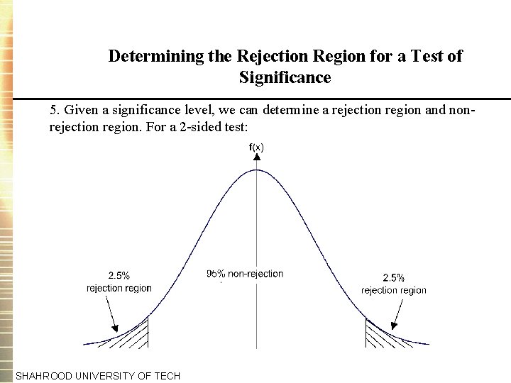
Determining the Rejection Region for a Test of Significance 5. Given a significance level, we can determine a rejection region and nonrejection region. For a 2 -sided test: SHAHROOD UNIVERSITY OF TECH

The Rejection Region for a 1 -Sided Test (Upper Tail) SHAHROOD UNIVERSITY OF TECH

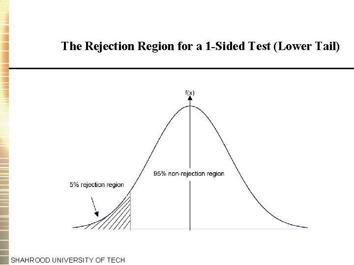
The Rejection Region for a 1 -Sided Test (Lower Tail) SHAHROOD UNIVERSITY OF TECH

The Test of Significance Approach: Drawing Conclusions 6. Use the t-tables to obtain a critical value or values with which to compare the test statistic. 7. Finally perform the test. If the test statistic lies in the rejection region then reject the null hypothesis (H 0), else do not reject H 0. SHAHROOD UNIVERSITY OF TECH

A Note on the t and the Normal Distribution • You should all be familiar with the normal distribution and its characteristic “bell” shape. • We can scale a normal variate to have zero mean and unit variance by subtracting its mean and dividing by its standard deviation. • There is, however, a specific relationship between the t- and the standard normal distribution. Both are symmetrical and centred on zero. The t-distribution has another parameter, its degrees of freedom. We will always know this (for the time being from the number of observations -2). SHAHROOD UNIVERSITY OF TECH

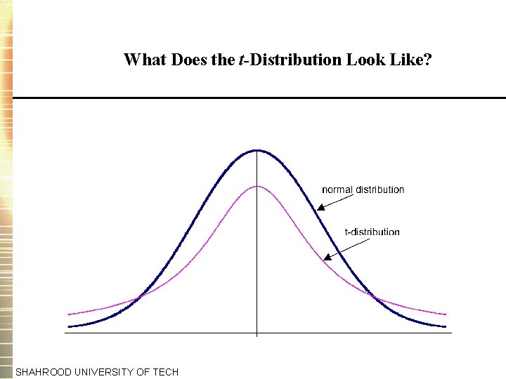
What Does the t-Distribution Look Like? SHAHROOD UNIVERSITY OF TECH

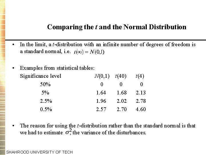
Comparing the t and the Normal Distribution • In the limit, a t-distribution with an infinite number of degrees of freedom is a standard normal, i. e. • Examples from statistical tables: Significance level N(0, 1) t(40) 50% 0 0 5% 1. 64 1. 68 2. 5% 1. 96 2. 02 0. 5% 2. 57 2. 70 t(4) 0 2. 13 2. 78 4. 60 • The reason for using the t-distribution rather than the standard normal is that we had to estimate , the variance of the disturbances. SHAHROOD UNIVERSITY OF TECH

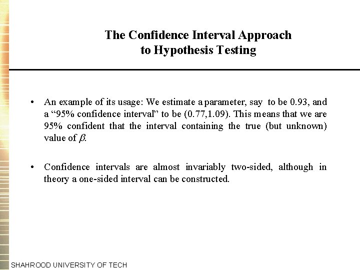
The Confidence Interval Approach to Hypothesis Testing • An example of its usage: We estimate a parameter, say to be 0. 93, and a “ 95% confidence interval” to be (0. 77, 1. 09). This means that we are 95% confident that the interval containing the true (but unknown) value of . • Confidence intervals are almost invariably two-sided, although in theory a one-sided interval can be constructed. SHAHROOD UNIVERSITY OF TECH

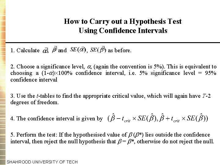
How to Carry out a Hypothesis Test Using Confidence Intervals 1. Calculate , and , as before. 2. Choose a significance level, , (again the convention is 5%). This is equivalent to choosing a (1 - ) 100% confidence interval, i. e. 5% significance level = 95% confidence interval 3. Use the t-tables to find the appropriate critical value, which will again have T-2 degrees of freedom. 4. The confidence interval is given by 5. Perform the test: If the hypothesised value of ( *) lies outside the confidence interval, then reject the null hypothesis that = *, otherwise do not reject the null. SHAHROOD UNIVERSITY OF TECH

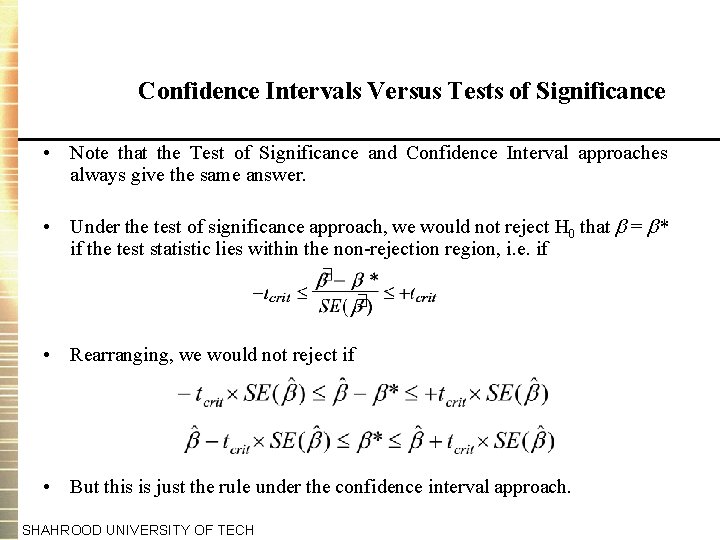
Confidence Intervals Versus Tests of Significance • Note that the Test of Significance and Confidence Interval approaches always give the same answer. • Under the test of significance approach, we would not reject H 0 that = * if the test statistic lies within the non-rejection region, i. e. if • Rearranging, we would not reject if • But this is just the rule under the confidence interval approach. SHAHROOD UNIVERSITY OF TECH

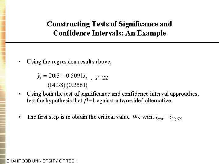
Constructing Tests of Significance and Confidence Intervals: An Example • Using the regression results above, , T=22 • Using both the test of significance and confidence interval approaches, test the hypothesis that =1 against a two-sided alternative. • The first step is to obtain the critical value. We want tcrit = t 20; 5% SHAHROOD UNIVERSITY OF TECH

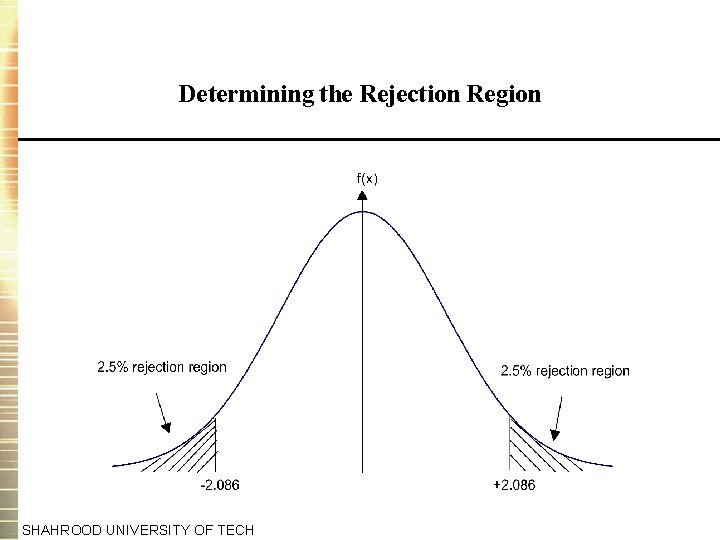
Determining the Rejection Region SHAHROOD UNIVERSITY OF TECH

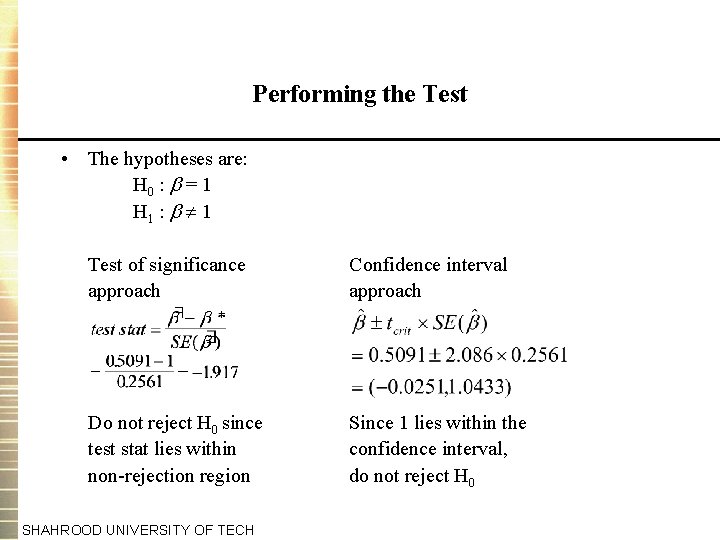
Performing the Test • The hypotheses are: H 0 : = 1 H 1 : 1 Test of significance approach Confidence interval approach Do not reject H 0 since test stat lies within non-rejection region Since 1 lies within the confidence interval, do not reject H 0 SHAHROOD UNIVERSITY OF TECH

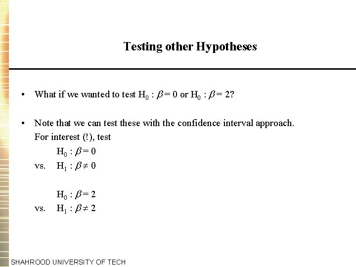
Testing other Hypotheses • What if we wanted to test H 0 : = 0 or H 0 : = 2? • Note that we can test these with the confidence interval approach. For interest (!), test H 0 : = 0 vs. H 1 : 0 vs. H 0 : = 2 H 1 : 2 SHAHROOD UNIVERSITY OF TECH

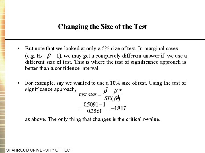
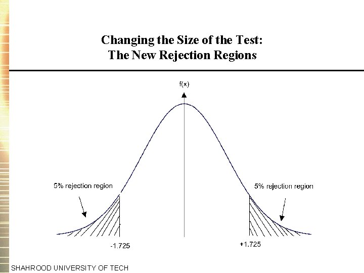
Changing the Size of the Test • But note that we looked at only a 5% size of test. In marginal cases (e. g. H 0 : = 1), we may get a completely different answer if we use a different size of test. This is where the test of significance approach is better than a confidence interval. • For example, say we wanted to use a 10% size of test. Using the test of significance approach, as above. The only thing that changes is the critical t-value. SHAHROOD UNIVERSITY OF TECH

Changing the Size of the Test: The New Rejection Regions SHAHROOD UNIVERSITY OF TECH

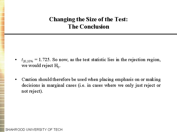
Changing the Size of the Test: The Conclusion • t 20; 10% = 1. 725. So now, as the test statistic lies in the rejection region, we would reject H 0. • Caution should therefore be used when placing emphasis on or making decisions in marginal cases (i. e. in cases where we only just reject or not reject). SHAHROOD UNIVERSITY OF TECH

Some More Terminology • If we reject the null hypothesis at the 5% level, we say that the result of the test is statistically significant. • Note that a statistically significant result may be of no practical significance. E. g. if a shipment of cans of beans is expected to weigh 450 g per tin, but the actual mean weight of some tins is 449 g, the result may be highly statistically significant but presumably nobody would care about 1 g of beans. SHAHROOD UNIVERSITY OF TECH

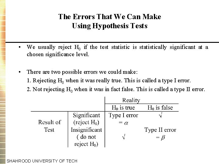
The Errors That We Can Make Using Hypothesis Tests • We usually reject H 0 if the test statistic is statistically significant at a chosen significance level. • There are two possible errors we could make: 1. Rejecting H 0 when it was really true. This is called a type I error. 2. Not rejecting H 0 when it was in fact false. This is called a type II error. SHAHROOD UNIVERSITY OF TECH

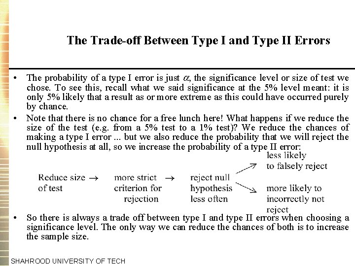
The Trade-off Between Type I and Type II Errors • The probability of a type I error is just , the significance level or size of test we chose. To see this, recall what we said significance at the 5% level meant: it is only 5% likely that a result as or more extreme as this could have occurred purely by chance. • Note that there is no chance for a free lunch here! What happens if we reduce the size of the test (e. g. from a 5% test to a 1% test)? We reduce the chances of making a type I error. . . but we also reduce the probability that we will reject the null hypothesis at all, so we increase the probability of a type II error: • So there is always a trade off between type I and type II errors when choosing a significance level. The only way we can reduce the chances of both is to increase the sample size. SHAHROOD UNIVERSITY OF TECH

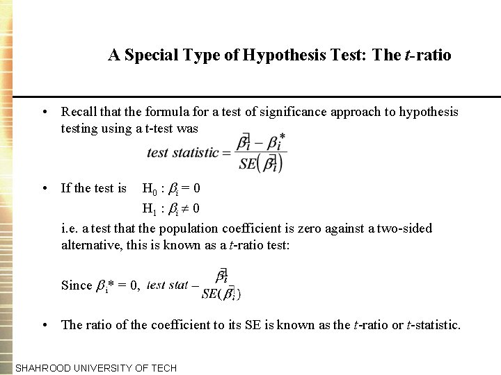
A Special Type of Hypothesis Test: The t-ratio • Recall that the formula for a test of significance approach to hypothesis testing using a t-test was H 0 : i = 0 H 1 : i 0 i. e. a test that the population coefficient is zero against a two-sided alternative, this is known as a t-ratio test: • If the test is Since i* = 0, • The ratio of the coefficient to its SE is known as the t-ratio or t-statistic. SHAHROOD UNIVERSITY OF TECH

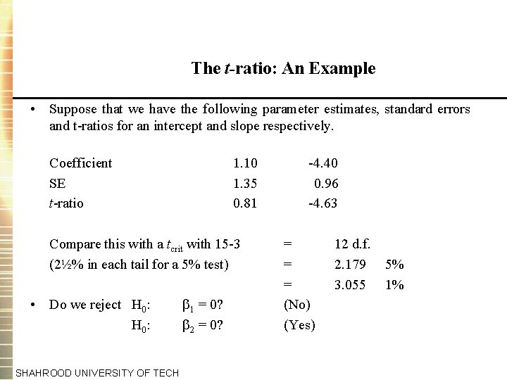
The t-ratio: An Example • Suppose that we have the following parameter estimates, standard errors and t-ratios for an intercept and slope respectively. Coefficient SE t-ratio 1. 10 1. 35 0. 81 Compare this with a tcrit with 15 -3 (2½% in each tail for a 5% test) • Do we reject H 0: H 0 : SHAHROOD UNIVERSITY OF TECH 1 = 0? 2 = 0? -4. 40 0. 96 -4. 63 = = = (No) (Yes) 12 d. f. 2. 179 3. 055 5% 1%

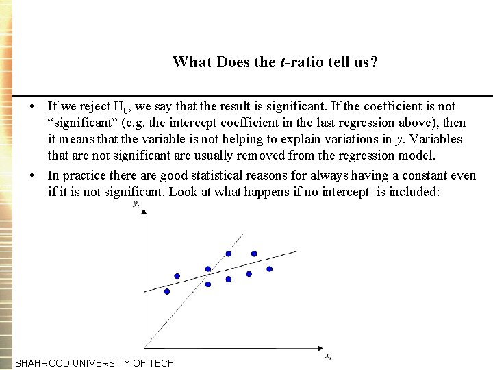
What Does the t-ratio tell us? • If we reject H 0, we say that the result is significant. If the coefficient is not “significant” (e. g. the intercept coefficient in the last regression above), then it means that the variable is not helping to explain variations in y. Variables that are not significant are usually removed from the regression model. • In practice there are good statistical reasons for always having a constant even if it is not significant. Look at what happens if no intercept is included: SHAHROOD UNIVERSITY OF TECH