A Brief Introduction to Logic Outline n n

A Brief Introduction to Logic - Outline n n n Propositional Logic : Syntax Propositional Logic : Semantics Satisfiability and validity Modeling with Propositional logic Normal forms Deductive proofs and resolution 1

Propositional logic n n A proposition – a sentence that can be either true or false. Propositions: n n x is greater than y Noam wrote this letter 2
:")
Propositional logic: Syntax n The symbols of the language: n n Propositional symbols (Prop): A, B, C, … Connectives: n n n n © , > and or not implies equivalent to xor (different than) False, True Parenthesis: (, ). 3

Propositional logic: Syntax n n Q 1: how many different binary symbols can we define ? Q 2: what is the minimal number of such symbols? 4

Formulas n Grammar of well-formed propositional formulas n Formula : = prop | ( Formula) | (Formula o Formula). n . . . where prop 2 Prop and o is one of the binary relations 5
 ( ( A))")
Formulas n Examples of well-formed formulas: n n n ( A) ( ( A)) (A (B C)) (A (B C)) Correct expressions of Propositional Logic are full of unnecessary parenthesis. 6

Formulas n n Abbreviations. We write Ao. Bo. Co… in place of (A o (B o (C o …))) Thus, we write A B C, A B C, … in place of (A (B C)), (A (B C)) 7

Formulas n n n We omit parenthesis whenever we may restore them through operator precedence: binds more strictly than , , and , bind more strictly than , . Thus, we write: A A B C for for ( ( A)), (( A ) B) ((A B) C), … 8

Alternative notations n n Negation: Conjunction: Clauses: Truth values: true/false 0/1
 of the operators")
Propositional Logic: Semantics n n Truth tables define the semantics (=meaning) of the operators Convention: 0 = false, 1 = true p 0 0 1 q 0 1 1 pÆq pÇq p!q 0 0 1 10
 of the operators p")
Propositional Logic: Semantics n Truth tables define the semantics (=meaning) of the operators p 0 0 1 q 0 1 1 : p p $ q p © q 1 1 0 0 0 1 1 0 11

Back to Q 1 n Q 1: How many binary operators can we define that have different semantic definition ? n A: 16 12

Assignments n n n Definition: A truth-values assignment, , is an element of 2 Prop (i. e. , 2 Prop). In other words, ® is a subset of the variables that are assigned true. Equivalently, we can see ® as a mapping from variables to truth values: : Prop {0, 1} n Example: ®: {A 0, B 1, . . . } 13
: intuition n n An assignment can either satisfy or not satisfy")
Satisfaction relation (²): intuition n n An assignment can either satisfy or not satisfy a given formula. ² φ means n n “ satisfies φ” or “ is a model of φ” We will first see an example. Then we will define these notions formally. 14
) Let ®")
Example n n n Let Á = (A Ç (B → C)) Let ® = {A 0, B 0, C 1} Q: Does ® satisfy Á? n n A: (0 Ç (0 → 1)) = (0 Ç 1) = 1 n n (in symbols: does it hold that ® ² Á ? ) Hence, ® ² Á. Let us now formalize an evaluation process. 15
: formalities n ² is a relation: ² µ (2 Prop")
The satisfaction relation (²): formalities n ² is a relation: ² µ (2 Prop x Formula) n Examples: n n ({a}, a Ç b) // the assignment ® = {a} satisfies a Ç b ({a, b}, a Æ b) 16
: formalities n ² is defined recursively: n n n ²")
The satisfaction relation (²): formalities n ² is defined recursively: n n n ² p if (p) = true ² φ if 2 φ. ² φ1 φ2 if ² φ1 and ² φ2 ² φ1 φ2 if ² φ1 or ² φ2 ² φ1 φ2 if ² φ1 implies ² φ2 ² φ1 φ2 if ² φ1 iff ² φ2 17

From definition to an evaluation algorithm n Truth Evaluation Problem n Given φ Formula and 2 AP(φ), does ² φ ? Eval(φ, ){ If φ A, return (A). If φ ( φ1) return Eval(φ1, )) If φ (φ1 o φ2) return Eval(φ1, ) o Eval(φ2, ) } n Eval uses polynomial time 18

It doesn’t give us more than what we already know. . . n Recall our example n n Let Á = (A Ç (B → C)) Let ® = {A 0, B 0, C 1} Eval(Á, ®) = Eval(A, ) Ç Eval(B → C, ) = 0 Ç Eval(B, ) → Eval(C, ) = 0 Ç (0 → 1) = 0 Ç 1 = 1 Hence, ® ² Á. 19
)")
We can now extend the truth table to formulas (p → (q → p)) (p Æ : p) p Ç : q p q 0 0 1 0 1 0 1 1 1 1 0 1 20

We can now extend the truth table to formulas x 1 x 2 x 3 x 1 → (x 2 → : x 3) 0 0 0 1 1 0 1 0 1 1 0 0 1 1 1 1 0 21

Set of assignments n n n Intuition: a formula specifies a set of truth assignments. Prop 2 Function models: Formula 2 (a formula set of satisfying assignments) Recursive definition: n n n models(A) = { | (A) = 1}, A Prop models( φ1) = 2 Prop – models(φ1) models(φ1 φ2) = models(φ1) models(φ2) models(φ1 φ2) = (2 Prop – models(φ1)) models(φ2) 22
 = {{10}, {01}, {11}} n This is compatible")
Example n models (A Ç B) = {{10}, {01}, {11}} n This is compatible with the recursive definition: models(A Ç B) = models(A) [ models (B) = {{10}, {11}} [ {{01}, {11}} = {{10}, {01}, {11}} 23

Theorem n Let φ Formula and 2 Prop, then the following statements are equivalent: 1. ² φ 2. models(φ) 24
 – the Atomic Propositions")
Only the projected assignment matters. . . n n AP(φ) – the Atomic Propositions in φ. Clearly AP(φ) µ Prop. Let 1, 2 2 Prop, φ Formula. Lemma: if 1|AP(φ) = 2|AP(φ) , then 1² φ iff 2 ² φ Projection Corollary: ² φ iff |AP(φ) ² φ n We will assume, for simplicity, that Prop = AP(φ). 25

Extension of ² to sets of assignments n Let φ 2 Formula n Let T be a set of assignments, i. e. , T 22 Prop n Definition. T ² φ if T models(φ) n i. e. , ² 22 Prop £ Formula n Examples: 26

Extension of ² to formulas n n ² 2 Formula £ 2 Formula Definition. Let 1, 2 be prop. formulas. 1 ² 2 iff models( 1) models( 2) iff for all 2 Prop if ² 1 then ² 2 Examples: x 1 Æ x 2 ² x 1 Ç x 2 x 1 Æ x 2 ² x 2 Ç x 3 27

Semantic Classification of formulas n n n A formula φ is called valid if models(φ) = 2 Prop. (also called a tautology). A formula φ is called satisfiable if models(φ) ; . A formula φ is called unsatisfiable if models(φ) = ; . (also called a contradiction). satisfiable unsatisfiable valid 28
)")
Validity, satisfiability. . . in truth tables p q (p → (q → q)) (p Æ : p) p Ç : q 0 0 1 0 1 0 1 1 1 1 0 1 29

Characteristics of valid/sat. formulas. . . n Lemma n n A formula φ is valid iff φ is unsatisfiable φ is satisfiable iff φ is not valid yes Is valid? ? Satisfiability checker no 30

Look what we can do now. . . n We can write: n ²Á when Á is valid n 2Á when Á is not valid n 2 : Á when Á is satisfiable n ² : Á when Á is unsatisfiable 31
 → (x 1 Ç x")
Examples n n n (x 1 Æ x 2) → (x 1 Ç x 2) → x 1 (x 1 Æ x 2) Æ : x 1 is is is valid satisfiable unsatisfiable 32

Time for equivalences n Here are some valid formulas: n n n ²AÆ1$A ²AÆ0$0 ² : : A $ A // The double-negation rule ² A Æ (B Ç C) $ (A Æ B) Ç (A Æ C) Some more (De-Morgan rules): n n ² : (A Æ B) $ (: A Ç : B) ² : (A Ç B) $ (: A Æ : B) 33

A minimal set of binary operators n n Recall the question: what is the minimal set of operators necessary? A: Through such equivalences all Boolean operators can be written with a single operator (NAND). n n Indeed, typically industrial circuits only use one type of logical gate We’ll see how two are enough: : and Æ n Or: Implies: Equivalence: n . . . n n ² (A Ç B) $ : (: A Æ : B) ² (A → B) $ (: A Ç B) ² (A $ B) $ (A → B) Æ (B → A) 34

The decision problem of formulas n The decision problem: Given a propositional formula Á, is Á satisfiable ? n An algorithm that always terminates with a correct answer to this problem is called a decision procedure for propositional logic. 35

A Brief Introduction to Logic - Outline n n n Propositional Logic : Syntax Propositional Logic : Semantics Satisfiability and validity Modeling with Propositional logic Normal forms Deductive proofs and resolution 36

Before we solve this problem. . . n n Q: Suppose we can solve the satisfiability problem. . . how can this help us? A: There are numerous problems in the industry that are solved via the satisfiability problem of propositional logic n n n Logistics. . . Planning. . . Electronic Design Automation industry. . . Cryptography. . . (every NP-P problem. . . ) 37

Example 1: placement of wedding guests n n n Three chairs in a row: 1, 2, 3 We need to place Aunt, Sister and Father. Constraints: n n Aunt doesn’t want to sit near Father Aunt doesn’t want to sit in the left chair Sister doesn’t want to sit to the right of Father Q: Can we satisfy these constraints? 38
 n Denote: Aunt = 1, Sister = 2, Father = 3")
Example 1 (cont’d) n Denote: Aunt = 1, Sister = 2, Father = 3 Introduce a propositional variable for each pair (person, place). xij = person i is sited in place j, for 1 · i, j · 3 n Constraints: n n n Aunt doesn’t want to sit near Father: ((x 1, 1 Ç x 1, 3) → : x 3, 2) Æ (x 1, 2 → (: x 3, 1 Æ : x 3, 3)) Aunt doesn’t want to sit in the left chair : x 1, 1 Sister doesn’t want to sit to the right of Father x 3, 1 → : x 2, 2 Æ x 3, 2 → : x 2, 3 39
 n More constraints: n Each person is placed: (x 1, 1")
Example 1 (cont’d) n More constraints: n Each person is placed: (x 1, 1 Ç x 1, 2 Ç x 1, 3) Æ (x 2, 1 Ç x 2, 2 Ç x 2, 3) Æ (x 3, 1 Ç x 3, 2 Ç x 3, 3) Or, more concisely: n No person is placed in more than one place: n n Overall 9 variables, 26 conjoined constraints. 40
 n n (1) All the dated letters in this room")
Example 2 (Lewis Carroll) n n (1) All the dated letters in this room are written on blue paper; (2) None of them are in black ink, except those that are written in the third person; (3) I have not filed any of them that I can read; (4) None of them, that are written on one sheet, are undated; (5) All of them, that are not crossed, are in black ink; (6) All of them, written by Brown, begin with "Dear Sir"; (7) All of them, written on blue paper, are filed; (8) None of them, written on more than one sheet, are crossed; (9) None of them, that begins with "Dear Sir", are written in the third person. Therefore, I cannot read any of Brown’s letters. Is this statement valid ? 41
 n n p = “the letter is dated” q = “the")
Example 2 (cont’d) n n p = “the letter is dated” q = “the letter is written on blue paper” (1) All the dated letters in this room are written on blue paper; p!q n n r = “the letter is written in black ink” s = “the letter is written in the third person” (2) None of them are in black ink, except those that are written in the third person; : s → : r n . . . 42

Example 3: assignment of frequencies n n n radio stations For each assign one of k transmission frequencies, k < n. E -- set of pairs of stations, that are too close to have the same frequency. Q: which graph problem does this remind you of ? 43
 n xi, j – station i is assigned frequency j, for")
Example 3 (cont’d) n xi, j – station i is assigned frequency j, for 1 · i · n, 1 · j · k. n Every station is assigned at least one frequency: n Every station is assigned not more than one frequency: n Close stations are not assigned the same frequency. For each (i, j) 2 E, 44

A Brief Introduction to Logic - Outline n n n n Brief historical notes on logic Propositional Logic : Syntax Propositional Logic : Semantics Satisfiability and validity Modeling with Propositional logic Normal forms Deductive proofs and resolution 47

Definitions… n n Definition: A literal is either an atom or a negation of an atom. Let = : (A Ç : B). Then: n n n Atoms: AP( ) = {A, B} Literals: lit( ) = {A, : B} Equivalent formulas can have different literals n n = : (A Ç : B) = : A Æ B Now lit( ) = {: A, B} 48

Definitions… n Definition: a term is a conjunction of literals n n Example: (A Æ : B Æ C) Definition: a clause is a disjunction of literals n Example: (A Ç : B Ç C) 49
 n n Definition: A formula is said to be in")
Negation Normal Form (NNF) n n Definition: A formula is said to be in Negation Normal Form (NNF) if it only contains : , Æ and Ç connectives and only atoms can be negated. Examples: n n 1 = : (A Ç : B) 2 = : A Æ B is not in NNF is in NNF 50

Converting to NNF n Every formula can be converted to NNF in linear time: n n n Eliminate all connectives other than Æ, Ç, : Use De Morgan and double-negation rules to push negations to the right Example: = : (A ! : B) n n n Eliminate ‘!’: = : (: A Ç : B) Push negation using De Morgan: = (: : A Æ : : B) Use Double negation rule: = (A Æ B) 51
 n Definition: A formula is said to be in Disjunctive")
Disjunctive Normal Form (DNF) n Definition: A formula is said to be in Disjunctive Normal Form (DNF) if it is a disjunction of terms. n In other words, it is a formula of the form where li, j is the j-th literal in the i-th term. n Examples n n = (A Æ : B Æ C) Ç (: A Æ D) Ç (B) is in DNF is a special case of NNF 52

Converting to DNF n Every formula can be converted to DNF in exponential time and space: n n n Convert to NNF Distribute disjunctions following the rule: ² A Æ (B Ç C) $ ((A Æ B) Ç (A Æ C)) Example: n n = (A Ç B) Æ (: C Ç D) = ((A Ç B) Æ (: C)) Ç ((A Ç B) Æ D) = (A Æ : C) Ç (B Æ : C) Ç (A Æ D) Ç (B Æ D) Q: how many clauses would the DNF have had we started from a conjunction of n clauses ? 53

Satisfiability of DNF n Is the following DNF formula satisfiable? (x 1 Æ x 2 Æ : x 1) Ç (x 2 Æ : x 3 Æ x 3) n What is the complexity of satisfiability of DNF formulas? 54
 n Definition: A formula is said to be in Conjunctive")
Conjunctive Normal Form (CNF) n Definition: A formula is said to be in Conjunctive Normal Form (CNF) if it is a conjunction of clauses. n In other words, it is a formula of the form where li, j is the j-th literal in the i-th term. n Examples n n = (A Ç : B Ç C) Æ (: A Ç D) Æ (B) is in CNF is a special case of NNF 55

Converting to CNF n Every formula can be converted to CNF: n n In exponential time and space with the same set of variables. In linear time and space if new variables are added. n n In this case the original and converted formulas are “equisatisfiable”. This technique is called Tseitin’s encoding. 56
 { case is a literal: return")
Converting to CNF: the exponential way CNF( ) { case is a literal: return is 1 Æ 2: return CNF( 1) Æ CNF( 2) is 1 Ç 2: return Dist(CNF( 1), CNF( 2)) } Dist( 1, 2) { case 1 is 11 Æ 12: return Dist( 11, 2) Æ Dist( 12, 2) 2 is 21 Æ 22: return Dist( 1, 21) Æ Dist( 1, 22) else: return 1 Ç 2 57

Converting to CNF: the exponential way n n n Consider the formula = (x 1 Æ y 1) Ç (x 2 Æ y 2) CNF( )= (x 1 Ç x 2) Æ (x 1 Ç y 2) Æ (y 1 Ç x 2) Æ (y 1 Ç y 2) Now consider: n = (x 1 Æ y 1) Ç (x 2 Æ y 2) Ç Ç (xn Æ yn) Q: How many clauses CNF( ) returns ? A: 2 n 58

Converting to CNF: Tseitin’s encoding n n Consider the formula = (A ! (B Æ C)) The parse tree: ! A Æ B n n n a 1 a 2 C Associate a new auxiliary variable with each gate. Add constraints that define these new variables. Finally, enforce the root node. 59

Converting to CNF: Tseitin’s encoding n Need to satisfy: (a 1 $ (A ! a 2)) Æ (a 2 $ (B Æ C)) Æ (a 1) ! A Æ B n a 1 a 2 C Each such constraint has a CNF representation with 3 or 4 clauses. 60

Converting to CNF: Tseitin’s encoding n Need to satisfy: (a 1 $ (A ! a 2)) Æ (a 2 $ (B Æ C)) Æ (a 1) n n First: (a 1 Ç A) Æ (a 1 Ç : a 2) Æ (: a 1 Ç : A Ç a 2) Second: (: a 2 Ç B) Æ (: a 2 Ç C) Æ (a 2 Ç : B Ç : C) 61

Converting to CNF: Tseitin’s encoding n Let’s go back to n = (x 1 Æ y 1) Ç (x 2 Æ y 2) Ç Ç (xn Æ yn) n With Tseitin’s encoding we need: n n 2 n auxiliary variables a 1, …, a 2 n. Each adds 3 constraints. Top clause: (a 1 Ç Ç an) Hence, we have n n 6 n + 1 clauses, instead of 2 n. 4 n variables rather than 2 n. 62

But we can do better… n 63

What now? n Time to solve the decision problem for propositional logic. n The only algorithm we saw so far was building truth tables. 64

Two classes of algorithms for validity n Q: Is φ valid ? n n Two classes of algorithm for finding out: 1. 2. n Equivalently: is : φ satisfiable? Enumeration of possible solutions (Truth tables etc). Deduction In general (beyond propositional logic): n n Enumeration is possible only in some theories. Deduction typically cannot be fully automated. 65
")
The satisfiability Problem: enumeration n Given a formula φ, is φ satisfiable? Boolean SAT(φ) { B: =false for all 2 AP(φ) B = B Eval(φ, ) end return B } n NP-Complete (the first-ever! – Cook’s theorem) 66

A Brief Introduction to Logic - Outline n n n n Brief historical notes on logic Propositional Logic : Syntax Propositional Logic : Semantics Satisfiability and validity Modeling with Propositional logic Normal forms Deductive proofs and resolution 67

Deduction requires axioms and Inference rules n Inference rules: n Antecedents Consequent Examples: A!B B!C A!B A B (rule-name) (trans) (M. P. ) 68

Axioms n Axioms are inference rules with no antecedents, e. g. , A ! (B ! A) n n (H 1) We can turn an inference rule into an axiom if we have ‘→’ in the logic. So the difference between them is not sharp. 69

Proofs n n n A proof uses a given set of inference rules and axioms. This is called the proof system. Let H be a proof system. `H φ means: there is a proof of φ in system H whose premises are included in `H is called the provability relation. 70

Example n n Let H be the proof system comprised of the rules Trans and M. P. that we saw earlier. Does the following relation holds? 71

Deductive proof: example a ! b, b ! c, c ! d, d ! e, a `H e 1. a ! b 2. b ! c 3. a ! c 4. c ! d 5. d ! e 6. c ! e 7. a ! e 8. a 9. e premise 1, 2, Trans premise 4, 5, Trans 3, 6, Trans premise 3, 8. M. P. 72
 a!b b!c c!d d!e (trans) a!c c!e (trans) a!e a (M.")
Proof graph (DAG) a!b b!c c!d d!e (trans) a!c c!e (trans) a!e a (M. P. ) e Roots: premises 73

Proofs n n The problem: ` is a relation defined by syntactic transformations of the underlying proof system. For a given proof system H, n n n does ` conclude “correct” conclusions from premises ? Can we conclude all true statements with H? Correct with respect to what ? n With respect to the semantic definition of the logic. In the case of propositional logic truth tables gives us this. 74

Soundness and completeness n Let H be a proof system n Soundness of H: if `H φ then ² φ n Completeness of H : n How to prove soundness and completeness ? if ² φ then `H φ 75
 n Let H be (M. P) + the following")
Example: Hilbert axiom system (H) n Let H be (M. P) + the following axiom schemas: A ! (B ! A) (H 1) ((A !(B ! C)) !((A! B)!(A! C)) (: B ! : A) ! (A ! B) n (H 2) (H 3) H is sound and complete 76

Soundness and completeness n n To prove soundness of H, prove the soundness of its axioms and inference rules (easy with truth-tables). For example: A 0 0 1 B 0 1 0 A ! (B ! A) 1 1 1 Completeness – harder, but possible. 77

The resolution inference system n The resolution inference rule for CNF: n Example: 78
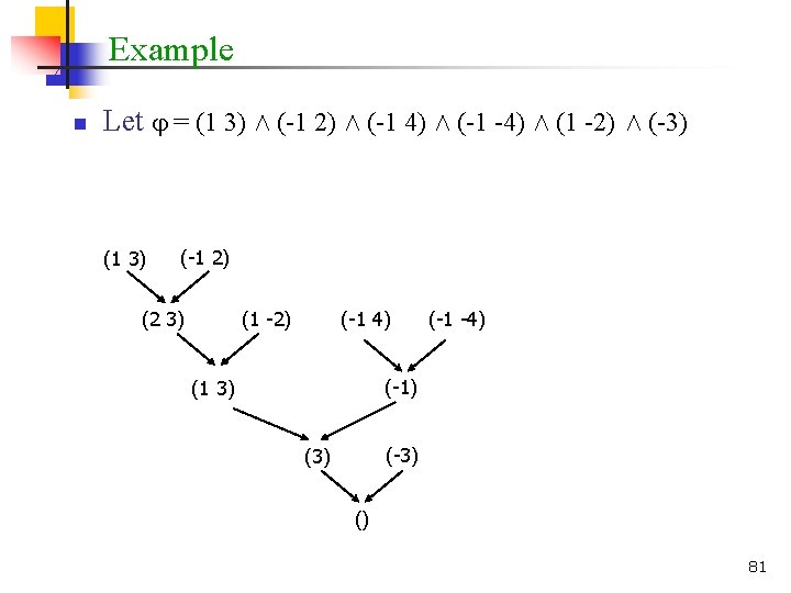
 Æ (-1 2 5) Æ")
Proof by resolution n n Let = (1 3) Æ (-1 2 5) Æ (-1 4) Æ (-1 -4) Æ (1 -2) We’ll try to prove → (3 5) (1 3) (-1 2 5) (2 3 5) (1 -2) (-1 4) (-1 -4) (-1) (1 3 5) (3 5) 79

Resolution n n Resolution is a sound and complete inference system for CNF If the input formula is unsatisfiable, there exists a proof of the empty clause 80
- Slides: 79