A Brief Introduction to CMAQ Serena H Chung

A Brief Introduction to CMAQ Serena H. Chung Bio. Earth Working Group 1 Seminar May 21, 2012

Outline • • • Chemical Transport Models (CTMs) CMAQ Model Components CMAQ Output Parallel Programming in CMAQ WRF and CMAQ Linkages

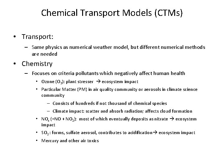
Chemical Transport Models (CTMs) • Transport: – Same physics as numerical weather model, but different numerical methods are needed • Chemistry – Focuses on criteria pollutants which negatively affect human health • Ozone (O 3): plant stresser ecosystem impact • Particular Matter (PM) in air quality community or aerosols in climate science community – Consists of hundreds if not thousand of chemical species – Climate impact: scatter and absorb radiation; affects cloud formation • NOx (=NO + NO 2): most of which eventually deposits as nitrate ecosystem impact • SO 2 : forms, sulfate aerosol, contributes to acidification ecosystem impact • Mercury and other air toxics

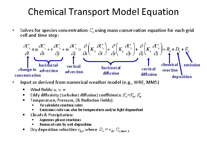
Chemical Transport Model Equation • Solves for species concentration Cs using mass conservation equation for each grid cell and time step: horizontal change in advection concentration • vertical advection horizontal diffusion chemical emission vertical reaction diffusion deposition Input or derived from numerical weather model (e. g. , WRF, MM 5) § § § Wind fields: u, v, w Eddy diffusivity (turbulent diffusion) coefficients: Kx=Ky, Kz Temperature, Pressure, (& Radiation Fields): § § To calculate reaction rates Emissions rate can also be temperature and/or light dependent § § Aqueous-phase reactions Removal rate by wet deposition Clouds & Precipitation: Dry deposition velocities vd, s, where Ds = vd, s Cs, layer 1

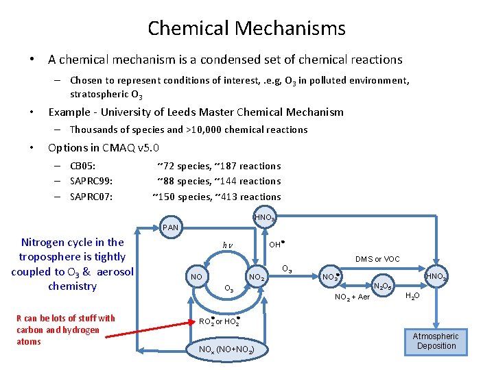
Chemical Mechanisms • A chemical mechanism is a condensed set of chemical reactions – Chosen to represent conditions of interest, . e. g, O 3 in polluted environment, stratospheric O 3 • Example - University of Leeds Master Chemical Mechanism – Thousands of species and >10, 000 chemical reactions • Options in CMAQ v 5. 0 – CB 05: – SAPRC 99: – SAPRC 07: ~72 species, ~187 reactions ~88 species, ~144 reactions ~150 species, ~413 reactions HNO 3 PAN Nitrogen cycle in the troposphere is tightly coupled to O 3 & aerosol chemistry R can be lots of stuff with carbon and hydrogen atoms OH● hn DMS or VOC NO NO 2 O 3 NO 3● NO 2 + Aer HNO 3 N 2 O 5 H 2 O ● ● RO 2 or HO 2 NOx (NO+NO 2) Atmospheric Deposition

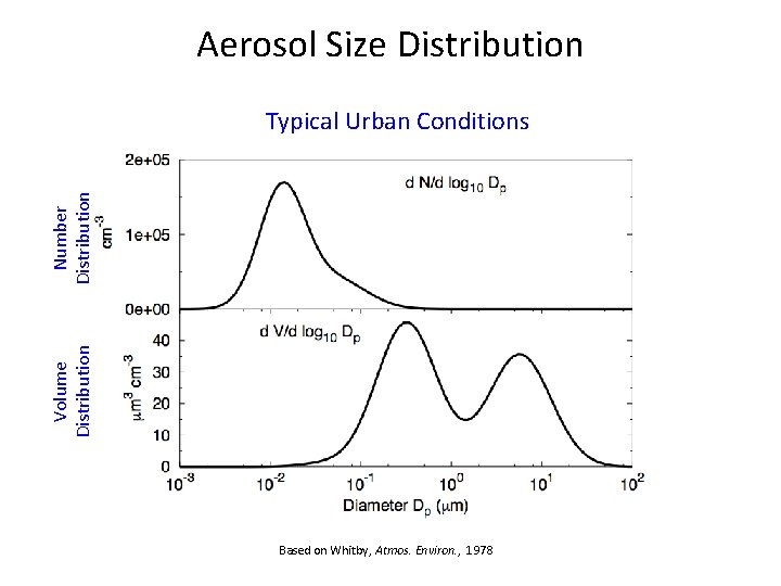
Aerosol Size Distribution Volume Distribution Number Distribution Typical Urban Conditions Based on Whitby, Atmos. Environ. , 1978

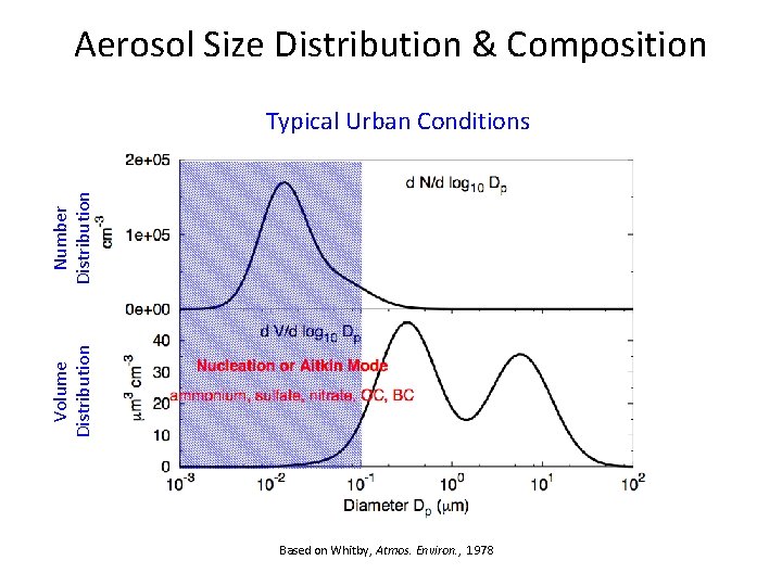
Aerosol Size Distribution & Composition Volume Distribution Number Distribution Typical Urban Conditions Based on Whitby, Atmos. Environ. , 1978

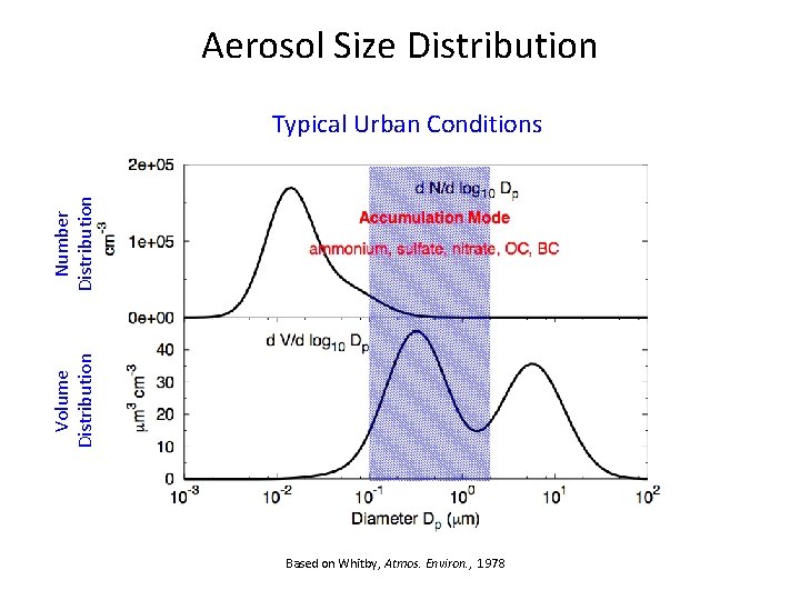
Aerosol Size Distribution Volume Distribution Number Distribution Typical Urban Conditions Based on Whitby, Atmos. Environ. , 1978

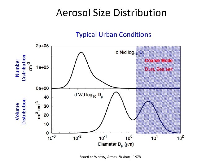
Aerosol Size Distribution Volume Distribution Number Distribution Typical Urban Conditions Based on Whitby, Atmos. Environ. , 1978

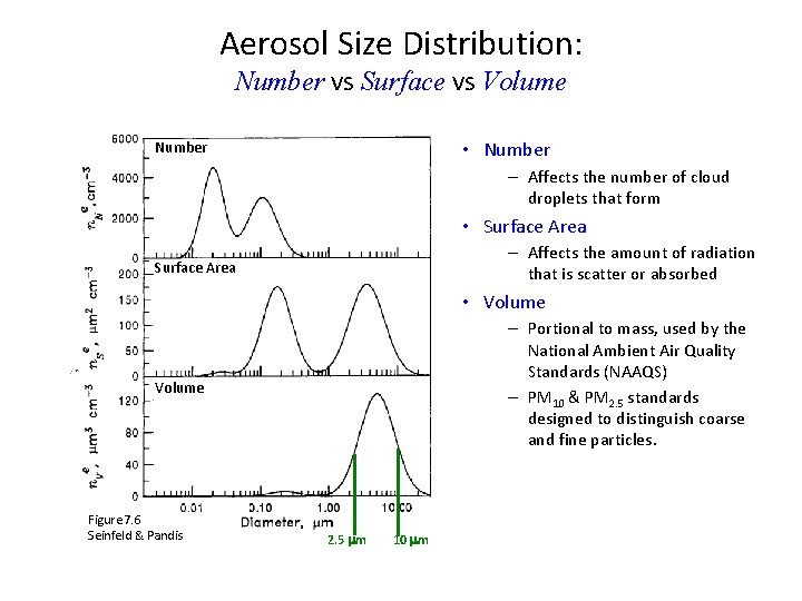
Aerosol Size Distribution: Number vs Surface vs Volume • Number – Affects the number of cloud droplets that form • Surface Area – Affects the amount of radiation that is scatter or absorbed Surface Area • Volume – Portional to mass, used by the National Ambient Air Quality Standards (NAAQS) – PM 10 & PM 2. 5 standards designed to distinguish coarse and fine particles. Volume Figure 7. 6 Seinfeld & Pandis 2. 5 mm 10 mm

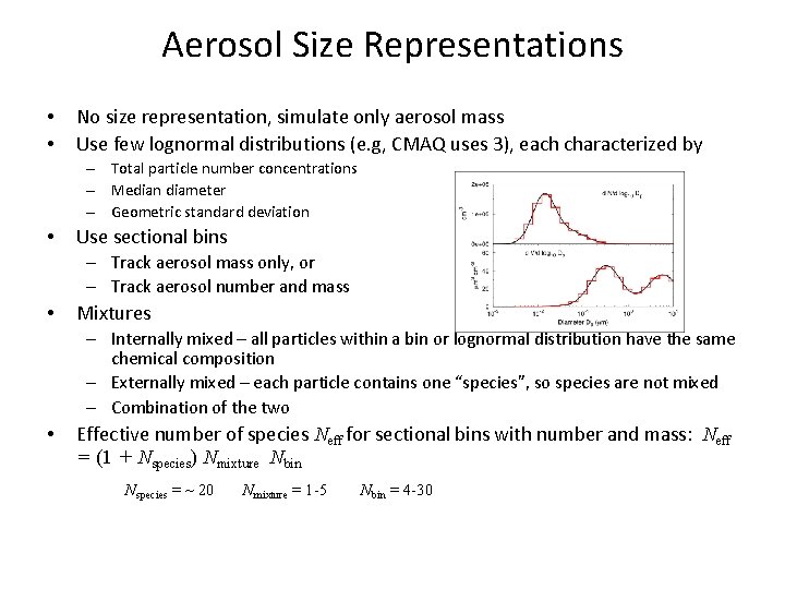
Aerosol Size Representations • • No size representation, simulate only aerosol mass Use few lognormal distributions (e. g, CMAQ uses 3), each characterized by – Total particle number concentrations – Median diameter – Geometric standard deviation • Use sectional bins – Track aerosol mass only, or – Track aerosol number and mass • Mixtures – Internally mixed – all particles within a bin or lognormal distribution have the same chemical composition – Externally mixed – each particle contains one “species”, so species are not mixed – Combination of the two • Effective number of species Neff for sectional bins with number and mass: Neff = (1 + Nspecies) Nmixture Nbin Nspecies = ~ 20 Nmixture = 1 -5 Nbin = 4 -30

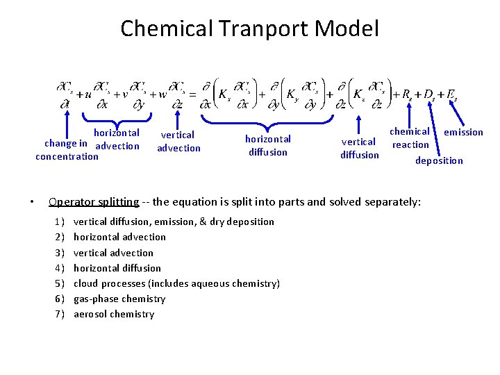
Chemical Tranport Model horizontal change in advection concentration • vertical advection horizontal diffusion chemical emission vertical reaction diffusion deposition Operator splitting -- the equation is split into parts and solved separately: 1) 2) 3) 4) 5) 6) 7) vertical diffusion, emission, & dry deposition horizontal advection vertical advection horizontal diffusion cloud processes (includes aqueous chemistry) gas-phase chemistry aerosol chemistry

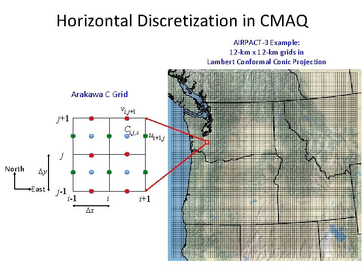
Horizontal Discretization in CMAQ AIRPACT-3 Example: 12 -km x 12 -km grids in Lambert Conformal Conic Projection Arakawa C Grid vi, j+1 Ci, j, s ui+1, j j North Dy East j-1 i Dx i+1

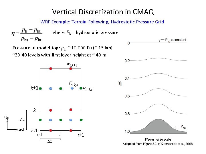
Vertical Discretization in CMAQ WRF Example: Terrain-Following, Hydrostatic Pressure Grid where Ph = hydrostatic pressure Pressure at model top: pht ~ 10, 000 Pa (~ 15 km) ~30 -40 levels with first layer height at ~ 40 m wi, k+1 Ci, k, s k+1 ui+1, j k Up Dh East k-1 i Dx i+1 Figure not to scale Adapted from Figure 2. 1 of Skamarock et al. , 2008

Vertical Discretization AIRPACT-4 Example

CMAQ Grid Cell in 3 -Dimension wi, j, k+1 vi, j+1, k ui+1, j, k ui, j, k Up vi, j/2, k North wi, j, k East Air density Temperature Pressure Water mixing ratios (vapor, rain, snow, ice) • Gas- and aerosol-phase chemical species mixing ratios • •

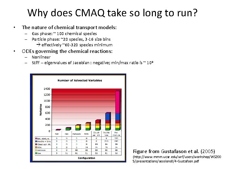
Why does CMAQ take so long to run? • The nature of chemical transport models: – Gas phase: ~ 100 chemical species – Particle phase: ~20 species, 3 -16 size bins effectively ~60 -320 species minimum • ODEs governing the chemical reactions: – Nonlinear – Stiff -- eigenvalues of Jacobian : negative; min/max ratio is ~ 109 Figure from Gustafason et al. (2005) (http: //www. mmm. ucar. edu/wrf/users/workshop/WS 200 5/presentations/sessions 8/4 -Gustafson. pdf

Model Time Steps • WRF: – Physics: recommendation is 6 seconds per km of Dx, i. e. , 72 seconds for 12 -km x 12 -km grids – Radiation: recommendation is 1 minute per km of Dx, i. e. , 12 minutes for 12 -km x 12 -km grids • CMAQ: – Synchronization between all processes: ~ 1 -3 min – Adaptive time step within each process

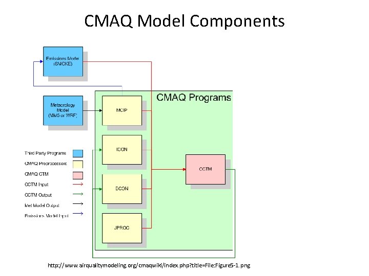
CMAQ Model Components http: //www. airqualitymodeling. org/cmaqwiki/index. php? title=File: Figure 5 -1. png

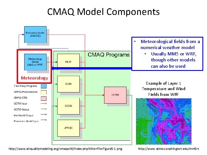
CMAQ Model Components • Meteorological fields from a numerical weather model • Usually MM 5 or WRF, though other models can also be used Meteorology http: //www. airqualitymodeling. org/cmaqwiki/index. php? title=File: Figure 5 -1. png Example of Layer 1 Temperature and Wind Fields from WRF http: //www. atmos. washington. edu/mm 5 rt

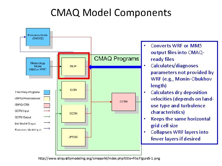
CMAQ Model Components • Converts WRF or MM 5 output files into CMAQready files • Calculates/diagnoses parameters not provided by WRF (e. g. , Monin-Obukhov length) • Calculates dry deposition velocities (depends on landuse type and turbulence characteristics) • Keeps the same horizontal grid cell size • Collapses WRF layers into fewer layers if desired http: //www. airqualitymodeling. org/cmaqwiki/index. php? title=File: Figure 5 -1. png

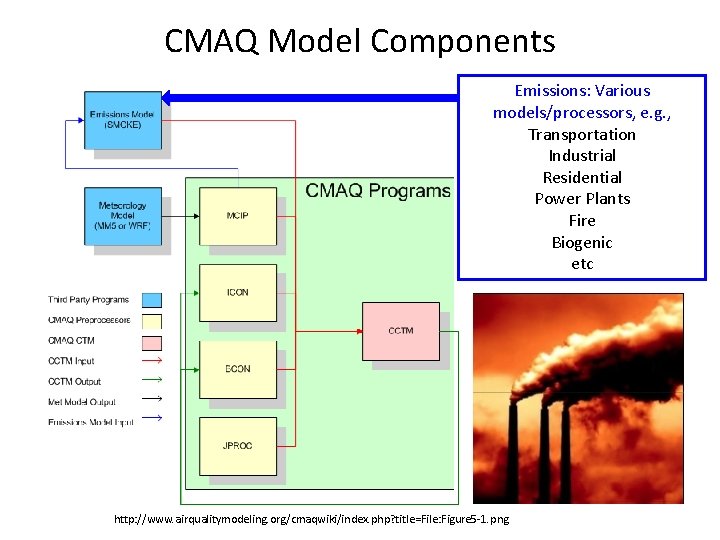
CMAQ Model Components Emissions: Various models/processors, e. g. , Transportation Industrial Residential Power Plants Fire Biogenic etc http: //www. airqualitymodeling. org/cmaqwiki/index. php? title=File: Figure 5 -1. png

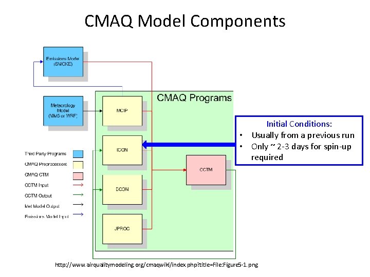
CMAQ Model Components Initial Conditions: • Usually from a previous run • Only ~ 2 -3 days for spin-up required http: //www. airqualitymodeling. org/cmaqwiki/index. php? title=File: Figure 5 -1. png

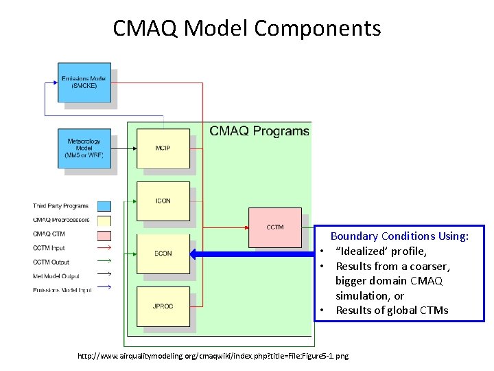
CMAQ Model Components Boundary Conditions Using: • “Idealized’ profile, • Results from a coarser, bigger domain CMAQ simulation, or • Results of global CTMs http: //www. airqualitymodeling. org/cmaqwiki/index. php? title=File: Figure 5 -1. png

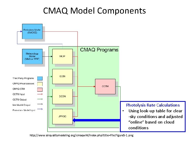
CMAQ Model Components Photolysis Rate Calculations • Using look-up table for clear -sky conditions and adjusted “online” based on cloud conditions http: //www. airqualitymodeling. org/cmaqwiki/index. php? title=File: Figure 5 -1. png

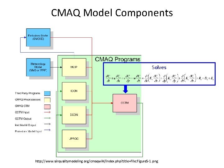
CMAQ Model Components Solves http: //www. airqualitymodeling. org/cmaqwiki/index. php? title=File: Figure 5 -1. png

CMAQ Output • Hourly, 3 -dimensional concentrations (. e. g, parts per billion or mg m-3) of chemical species • Hourly accumulated wet and dry deposition (. e. g, kg ha-1 hr-1) for relevant species • net. CDF files – same as WRF, but different conventions for date/time – read/write easier with use of Models-3 I/O API library • Examples: – http: //lar. wsu. edu/airpact/gmap/test. C. html

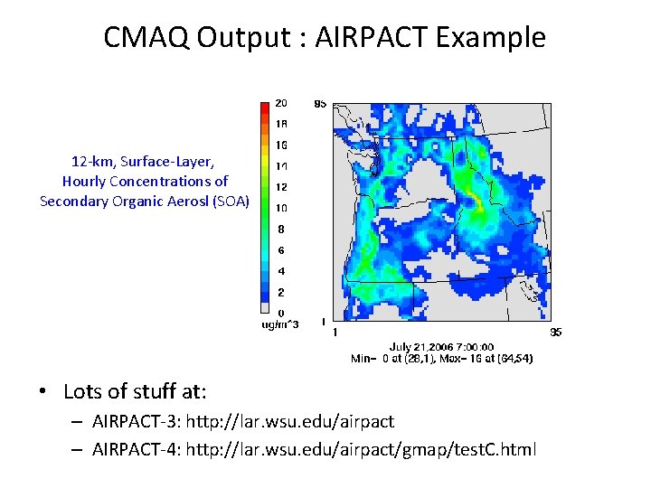
CMAQ Output : AIRPACT Example 12 -km, Surface-Layer, Hourly Concentrations of Secondary Organic Aerosl (SOA) • Lots of stuff at: – AIRPACT-3: http: //lar. wsu. edu/airpact – AIRPACT-4: http: //lar. wsu. edu/airpact/gmap/test. C. html

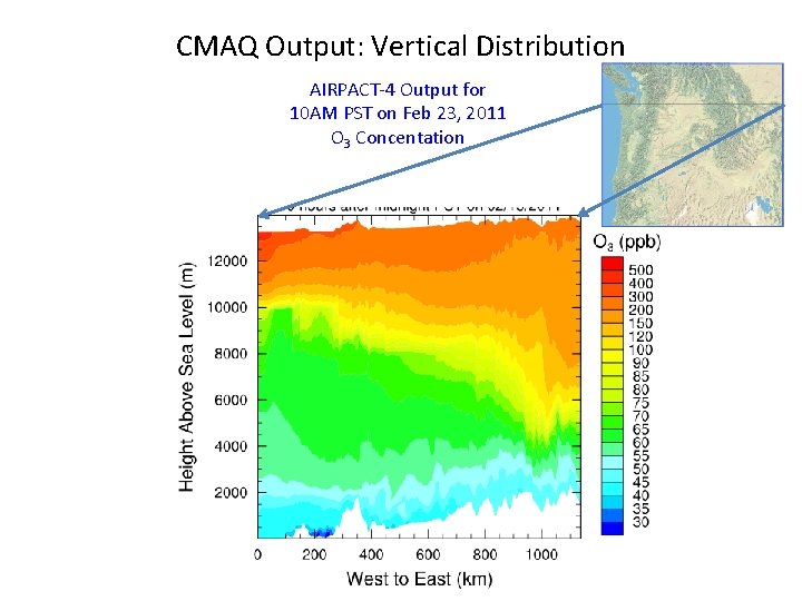
CMAQ Output: Vertical Distribution AIRPACT-4 Output for 10 AM PST on Feb 23, 2011 O 3 Concentation

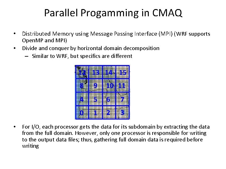
Parallel Progamming in CMAQ • Distributed Memory using Message Passing Interface (MPI) (WRF supports • Open. MP and MPI) Divide and conquer by horizontal domain decomposition – Similar to WRF, but specifics are different 12 13 14 15 • 8 9 10 11 4 5 6 7 0 1 2 3 For I/O, each processor gets the data for its subdomain by extracting the data from the full domain. However, only one processor is responsible for writing to the output data files; thus, gathering full domain data is required before writing

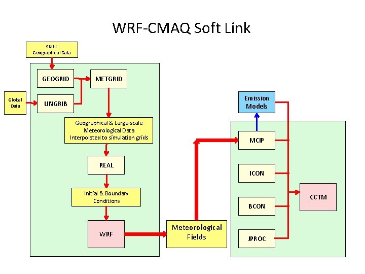
WRF-CMAQ Soft Link Static Geographical Data GEOGRID Global Data METGRID Emission Models UNGRIB Geographical & Large-scale Meteorological Data Interpolated to simulation grids MCIP REAL ICON Initial & Boundary Conditions WRF CCTM BCON Meteorological Fields JPROC

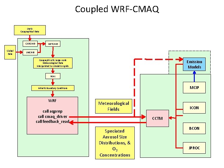
Coupled WRF-CMAQ Static Geographical Data GEOGRID Global Data METGRID UNGRIB Geographical & Large-scale Meteorological Data Interpolated to simulation grids Emission Models REAL MCIP Initial & Boundary Conditions WRF call aqprep call cmaq_driver call feedback_read Meteorological Fields ICON CCTM Speciated Aerosol Size Distributions, & O 3 Concentrations BCON JPROC

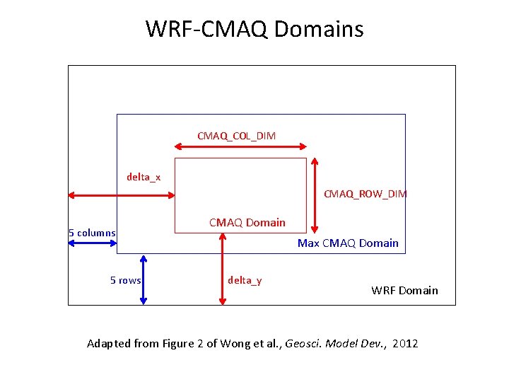
WRF-CMAQ Domains CMAQ_COL_DIM delta_x CMAQ_ROW_DIM 5 columns 5 rows CMAQ Domain Max CMAQ Domain delta_y WRF Domain Adapted from Figure 2 of Wong et al. , Geosci. Model Dev. , 2012

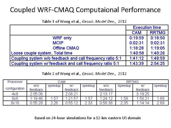
Coupled WRF-CMAQ Computaional Performance Table 1 of Wong et al. , Geosci. Model Dev. , 2012 WRF only MCIP Offline CMAQ Loose couple system, Total time Coupling system w/o feedback and call frequency ratio 5: 1 Coupling system w/ feedback and call frequency ratio 5: 1 Execution time CAM RRTMG 0: 19: 59 0: 18: 50 0: 02: 31 1: 18: 28 1: 19: 05 1: 40: 58 1: 40: 26 1: 41: 12 1: 48: 59 1: 43: 39 2: 54: 25 Table 2 of Wong et al. , Geosci. Model Dev. , 2012 Processor configuration w/o feedback CAM speedup w/ feedback 4 x 8 8 x 16 2: 05: 06 1: 19: 46 0: 55: 28 2: 08: 21 1: 21: 57 0: 55: 12 1. 57 2. 26 speedup 1. 57 2. 33 w/o feedback RRTMG Speedup w/ feedback 2: 13: 17 1: 24: 12 0: 56: 38 3: 19: 25 1: 58: 21 1: 14 1. 58 2. 35 Based on 24 -hour simulations for a 12 -km eastern US domain speedup 1. 68 2. 69

Some resources • • • http: //cmaq-model. org http: //cmascenter. org/ Seinfeld, J. H. and S. N. Pandis, Atmospheric Chemistry and Physics: From Air Pollution to Climate Change, John Wiley & Sons, 2006. Jacob, D. J. , Introduction to Atmospheric Chemistry, Princeton University Press, 1999. Jacobson, M. Z. , Fundamentals of Atmospheric Modeling, Cambridge University Press, 1999