A big advantage of classifiers is that the

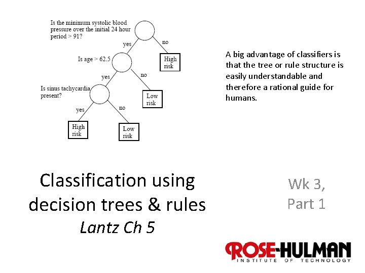
A big advantage of classifiers is that the tree or rule structure is easily understandable and therefore a rational guide for humans. Classification using decision trees & rules Wk 3, Part 1 Lantz Ch 5 1

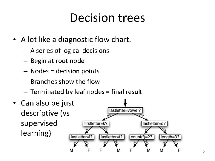
Decision trees • A lot like a diagnostic flow chart. – – – A series of logical decisions Begin at root node Nodes = decision points Branches show the flow Terminated by leaf nodes = final result • Can also be just descriptive (vs supervised learning) 2

A major branch of machine learning • The single most widely used method. – Can model almost any type of data. – Often provide accuracy and run fast. • Not so good if a large number of nominal features or a large number of numeric features. – Makes the “decision process” a big mess. 3

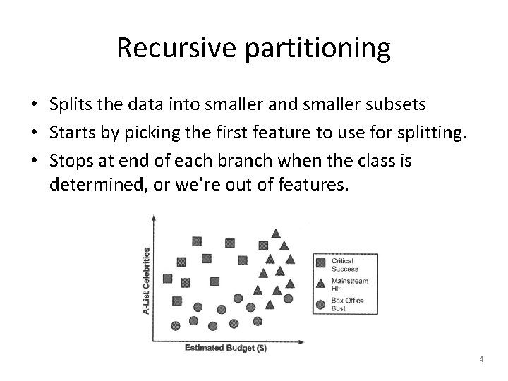
Recursive partitioning • Splits the data into smaller and smaller subsets • Starts by picking the first feature to use for splitting. • Stops at end of each branch when the class is determined, or we’re out of features. 4

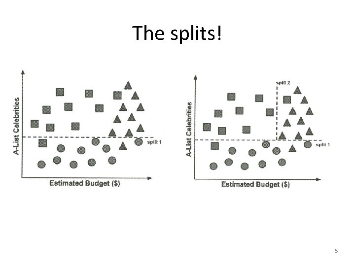
The splits! 5

Axis-parallel splits • Decision trees split data based on one criterion at a time. – Maybe some combination would have worked better? – Trade-off of A-list celebrities vs budget? 6

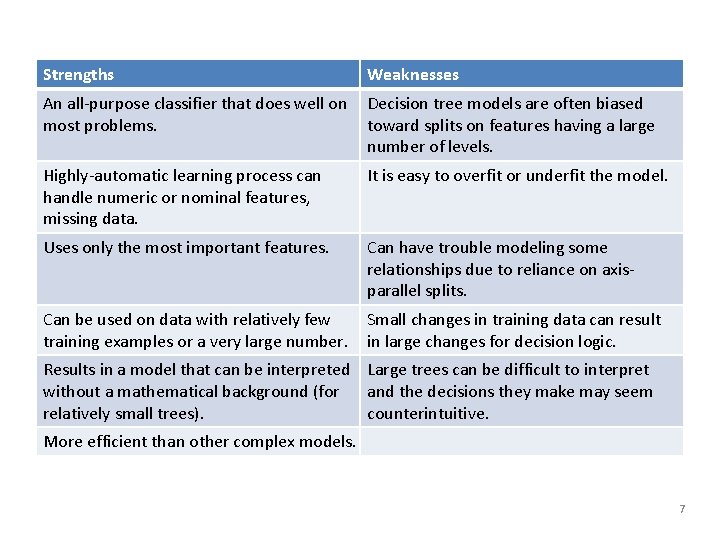
Strengths Weaknesses An all-purpose classifier that does well on most problems. Decision tree models are often biased toward splits on features having a large number of levels. Highly-automatic learning process can handle numeric or nominal features, missing data. It is easy to overfit or underfit the model. Uses only the most important features. Can have trouble modeling some relationships due to reliance on axisparallel splits. Can be used on data with relatively few training examples or a very large number. Small changes in training data can result in large changes for decision logic. Results in a model that can be interpreted Large trees can be difficult to interpret without a mathematical background (for and the decisions they make may seem relatively small trees). counterintuitive. More efficient than other complex models. 7

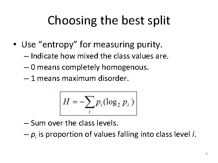
Choosing the best split • Use “entropy” for measuring purity. – Indicate how mixed the class values are. – 0 means completely homogenous. – 1 means maximum disorder. – Sum over the class levels. – pi is proportion of values falling into class level i. 8

Entropy example • A partition of data with two classes: – Red is 60% – White is 40% • Entropy is: -0. 60 * log 2(0. 60) -0. 40 * log 2(0. 40) = 0. 97. If this had been a 50/50 split, entropy would have been 1. 9

This comes out of Information Theory • Claude Shannon: “The goal of information is to reduce uncertainty. ” He also contributed to the ideas behind decision trees: The first notable use of decision trees was in EPAM, the "Elementary Perceiver And Memorizer” (Feigenbaum, 1961), which was a simulation of human concept learning_ IT)1 (Quinlan, 1979) added the crucial idea of choosing the attribute with maximum entropy; it is the basis for the [most common] decision tree algorithm. Information theory was developed by Claude Shannon to aid in the study of communication (Shannon and Weaver, 1949). (Shannon also contributed one of the earliest examples of machine learning, a mechanical mouse mimed Theseus that learned to navigate through a maze by trial and error. ) 10

How it works • The ID 3 algorithm builds the tree with the learning model like this: 1. Calculate the entropy of every attribute using the data set S 2. Split the set S into subsets using the attribute for which entropy is minimum (or, equivalently, information gain is maximum) 3. Make a decision tree node containing that attribute 4. Recurse on subsets using remaining attributes. 11

In pseudocode ID 3 (Examples, Target_Attribute, Attributes) Create a root node for the tree If all examples are positive, Return the single-node tree Root, with label = +. If all examples are negative, Return the single-node tree Root, with label = -. If number of predicting attributes is empty, then Return the single node tree Root, with label = most common value of the target attribute in the examples. Otherwise Begin A ← The Attribute that best classifies examples. Decision Tree attribute for Root = A. For each possible value, , of A, Add a new tree branch below Root, corresponding to the test A =. Let Examples() be the subset of examples that have the value for A If Examples() is empty Then below this new branch add a leaf node with label = most common target value in the examples Else below this new branch add the subtree ID 3 (Examples(), Target_Attribute, Attributes – {A}) End Return Root 12

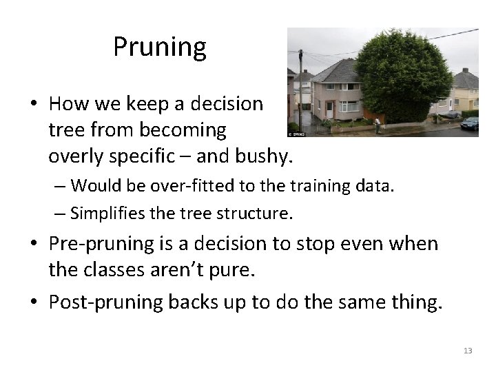
Pruning • How we keep a decision tree from becoming overly specific – and bushy. – Would be over-fitted to the training data. – Simplifies the tree structure. • Pre-pruning is a decision to stop even when the classes aren’t pure. • Post-pruning backs up to do the same thing. 13

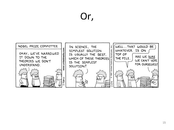
Major goals of decision trees • Come up with a parsimonious set of rules. • Occam’s razor and Minimum Description Length (MDL) are related: – The best hypothesis for a set of data is the one that leads to the best compression of the data. – Which neatly ties decision trees back to Information Theory. • A major goal of that was maximum compression. • Like, how to make the best use of telephone bandwidth. 14

Or, 15

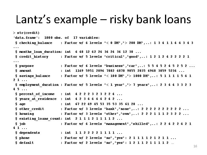
Lantz’s example – risky bank loans > str(credit) 'data. frame': 1000 obs. $ checking_balance : . . . $ months_loan_duration: $ credit_history : . . . $ purpose : $ amount : $ savings_balance : 2 1. . . $ employment_duration : 4 5. . . $ percent_of_income : $ years_at_residence : $ age : $ other_credit : $ housing : $ existing_loans_count: $ job : 4 1. . . $ dependents : $ phone : $ default : of 17 variables: Factor w/ 4 levels "< 0 DM", "> 200 DM", . . : 1 3 4 1 1 4 4 3 int 6 48 12 42 24 36 12 30. . . Factor w/ 5 levels "critical", "good", . . : 1 2 4 2 2 1 Factor w/ 6 levels "business", "car", . . : 5 5 4 5 2 5 2. . . int 1169 5951 2096 7882 4870 9055 2835 6948 3059 5234. . . Factor w/ 5 levels "< 100 DM", "> 1000 DM", . . : 5 1 1 5 4 1 Factor w/ 5 levels "< 1 year", "> 7 years", . . : 2 3 4 4 3 3 2 3 int 4 2 2 2 3 2 2 4. . . int 4 2 3 4 4 2 4 2. . . int 67 22 49 45 53 35 61 28. . . Factor w/ 3 levels "bank", "none", . . : 2 2 2 2 2. . . Factor w/ 3 levels "other", "own", . . : 2 2 2 1 1 1 2 3 2 2. . . int 2 1 1 1 1 2. . . Factor w/ 4 levels "management", "skilled", . . : 2 2 4 2 1 int 1 1 2 2 1 1. . . Factor w/ 2 levels "no", "yes": 2 1 1. . . Factor w/ 2 levels "no", "yes": 1 2 1 1 1 1 2 … 16

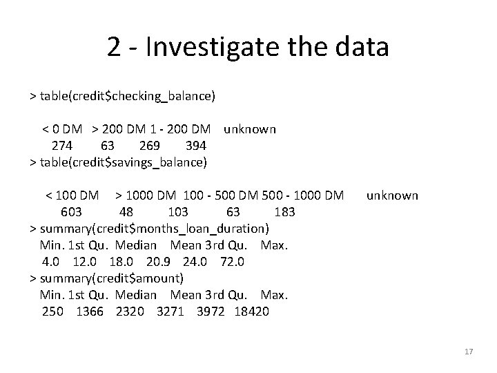
2 - Investigate the data > table(credit$checking_balance) < 0 DM > 200 DM 1 - 200 DM unknown 274 63 269 394 > table(credit$savings_balance) < 100 DM > 1000 DM 100 - 500 DM 500 - 1000 DM 603 48 103 63 183 > summary(credit$months_loan_duration) Min. 1 st Qu. Median Mean 3 rd Qu. Max. 4. 0 12. 0 18. 0 20. 9 24. 0 72. 0 > summary(credit$amount) Min. 1 st Qu. Median Mean 3 rd Qu. Max. 250 1366 2320 3271 3972 18420 unknown 17

Randomize the data examples! > set. seed(12345) >credit_rand <- credit[order(runif(1000), ] • Somehow, this “uniform” distribution doesn’t repeat or miss any rows. E. g. , > order(runif(10)) [1] 4 2 1 3 10 6 5 7 9 8 • Obviously important to make a new matrix! 18

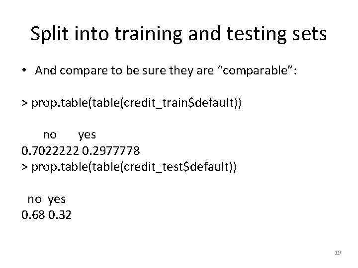
Split into training and testing sets • And compare to be sure they are “comparable”: > prop. table(credit_train$default)) no yes 0. 7022222 0. 2977778 > prop. table(credit_test$default)) no yes 0. 68 0. 32 19

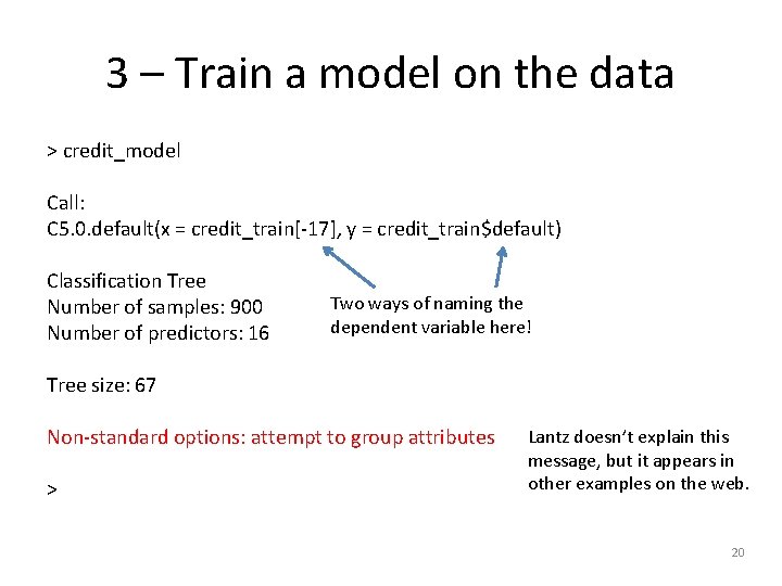
3 – Train a model on the data > credit_model Call: C 5. 0. default(x = credit_train[-17], y = credit_train$default) Classification Tree Number of samples: 900 Number of predictors: 16 Two ways of naming the dependent variable here! Tree size: 67 Non-standard options: attempt to group attributes > Lantz doesn’t explain this message, but it appears in other examples on the web. 20

Training results > summary(credit_model) Call: C 5. 0. default(x = credit_train[-17], y = credit_train$default) C 5. 0 [Release 2. 07 GPL Edition] ---------------- Fri Dec 12 07: 27 2014 Class specified by attribute `outcome' Read 900 cases (17 attributes) from undefined. data Decision tree: checking_balance = unknown: no (358/44) checking_balance in {< 0 DM, > 200 DM, 1 - 200 DM}: : . . . credit_history in {perfect, very good}: : . . . dependents > 1: yes (10/1) : dependents <= 1: : : . . . savings_balance = < 100 DM: yes (39/11) : savings_balance in {> 1000 DM, 500 - 1000 DM, unknown}: no (8/1) : savings_balance = 100 - 500 DM: : : . . . checking_balance = < 0 DM: no (1) : checking_balance in {> 200 DM, 1 - 200 DM}: yes (5/1 ) credit_history in {critical, good, poor}: : . . . months_loan_duration <= 11: no (87/14) months_loan_duration > 11: : . . . savings_balance = > 1000 DM: no (13) savings_balance in {< 100 DM, 100 - 500 DM, 500 - 1000 DM, unknown}: : . . . checking_balance = > 200 DM: : . . . dependents > 1: yes (3) : dependents <= 1: : : . . . credit_history in {good, poor}: no (23/3) : credit_history = critical: : : . . . amount <= 2337: yes (3) : amount > 2337: no (6) checking_balance = 1 - 200 DM: : . . . savings_balance = unknown: no (34/6) : savings_balance in {< 100 DM, 100 - 500 DM, 500 - 1000 DM}: If checking account balance is unknown, then classify as not likely to default! (But this was wrong in 44 of 358 cases. ) 21

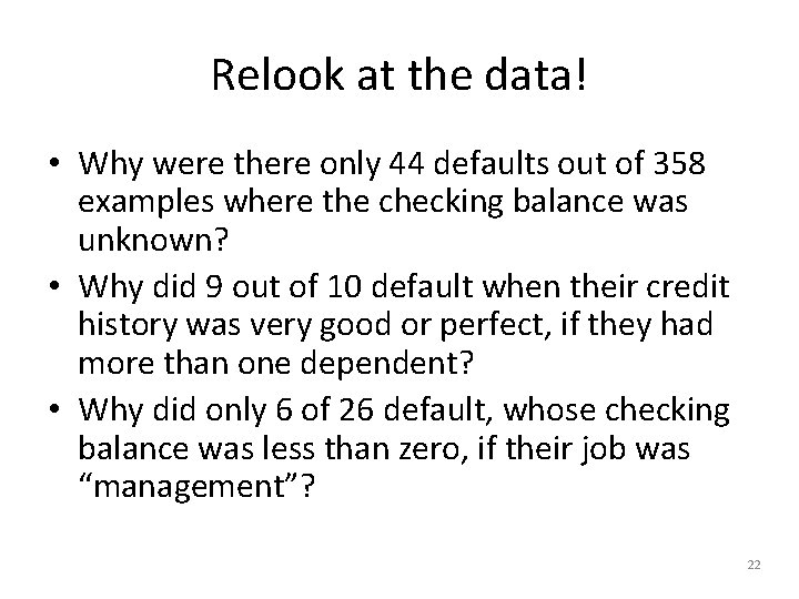
Relook at the data! • Why were there only 44 defaults out of 358 examples where the checking balance was unknown? • Why did 9 out of 10 default when their credit history was very good or perfect, if they had more than one dependent? • Why did only 6 of 26 default, whose checking balance was less than zero, if their job was “management”? 22

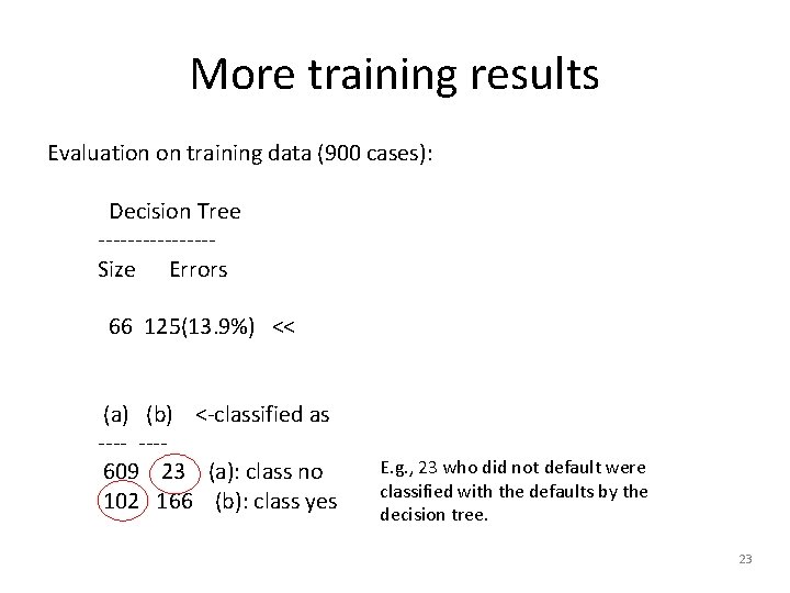
More training results Evaluation on training data (900 cases): Decision Tree --------Size Errors 66 125(13. 9%) << (a) (b) <-classified as ---- ---609 23 (a): class no 102 166 (b): class yes E. g. , 23 who did not default were classified with the defaults by the decision tree. 23

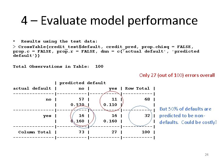
4 – Evaluate model performance • Results using the test data: > Cross. Table(credit_test$default, credit_pred, prop. chisq = FALSE, prop. c = FALSE, prop. r = FALSE, dnn = c('actual default', 'predicted default')) Total Observations in Table: 100 Only 27 (out of 100) errors overall | predicted default actual default | no | yes | Row Total | --------|-----------|------| no | 57 | 11 | 68 | | 0. 570 | 0. 110 | | --------|-----------|------| yes | 16 | 32 | | 0. 160 | | --------|-----------|------| Column Total | 73 | 27 | 100 | --------|-----------|------| But 50% of defaults are predicted to be nondefaults. Could be costly! 24

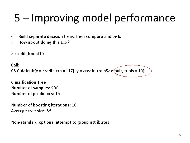
5 – Improving model performance • • Build separate decision trees, then compare and pick. How about doing this 10 x? > credit_boost 10 Call: C 5. 0. default(x = credit_train[-17], y = credit_train$default, trials = 10) Classification Tree Number of samples: 900 Number of predictors: 16 Number of boosting iterations: 10 Average tree size: 56 Non-standard options: attempt to group attributes 25

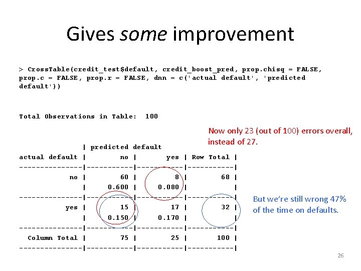
Gives some improvement > Cross. Table(credit_test$default, credit_boost_pred, prop. chisq = FALSE, prop. c = FALSE, prop. r = FALSE, dnn = c('actual default', 'predicted default')) Total Observations in Table: 100 Now only 23 (out of 100) errors overall, instead of 27. | predicted default actual default | no | yes | Row Total | --------|-----------|------| no | 60 | 8 | 68 | | 0. 600 | 0. 080 | | --------|-----------|------| yes | 15 | 17 | 32 | | 0. 150 | 0. 170 | | --------|-----------|------| Column Total | 75 | 25 | 100 | --------|-----------|------| But we’re still wrong 47% of the time on defaults. 26

A theoretical note… • We tried 10 variations on designing the tree, here, with the 10 trials. • There were 16 predictors in play. • To do an exhaustive job finding the MDL (Ref slide 12), we might need to try 216 designs! – Exponential complexity, that has. – And mostly, refining noise, we’d be. 27

New angle – Make some errors more costly! > error_cost [, 1] [, 2] Since a loan default [1, ] 0 4 costs 4 x as much as a missed opportunity. [2, ] 1 0 > credit_cost <- C 5. 0(credit_train[-17], credit_train$default, costs = error_cost) 28

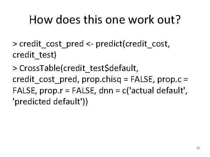
How does this one work out? > credit_cost_pred <- predict(credit_cost, credit_test) > Cross. Table(credit_test$default, credit_cost_pred, prop. chisq = FALSE, prop. c = FALSE, prop. r = FALSE, dnn = c('actual default', 'predicted default')) 29

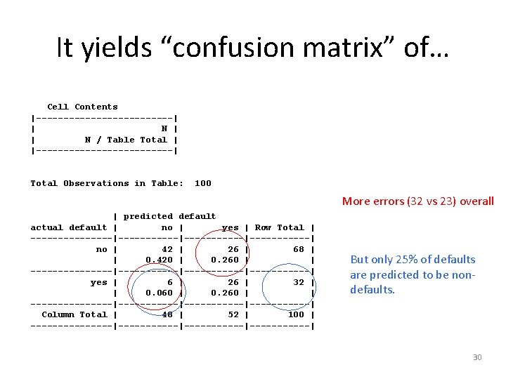
It yields “confusion matrix” of… Cell Contents |-------------| | N / Table Total | |-------------| Total Observations in Table: 100 More errors (32 vs 23) overall | predicted default actual default | no | yes | Row Total | --------|-----------|------| no | 42 | 26 | 68 | | 0. 420 | 0. 260 | | --------|-----------|------| yes | 6 | 26 | 32 | | 0. 060 | 0. 260 | | --------|-----------|------| Column Total | 48 | 52 | 100 | --------|-----------|------| But only 25% of defaults are predicted to be nondefaults. 30

New topic – Classification Rules • Vs trees • Separate and conquer is the strategy. • Identify a rule that covers a subset, then pull those out and look at the rest. • Keep adding rules till the whole dataset has been covered. • Emphasis is on finding rules to identify every example which passes some test. 31

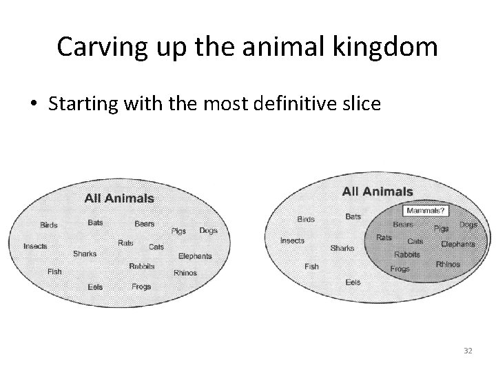
Carving up the animal kingdom • Starting with the most definitive slice 32

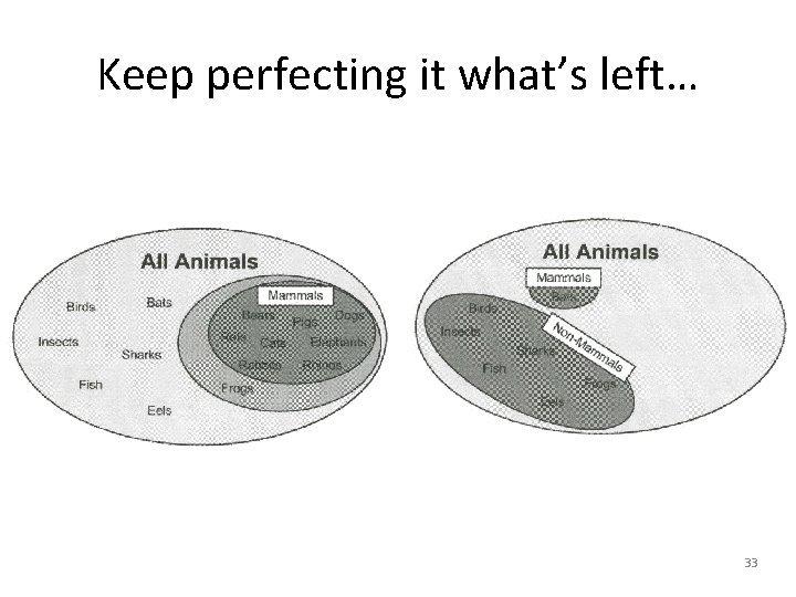
Keep perfecting it what’s left… 33

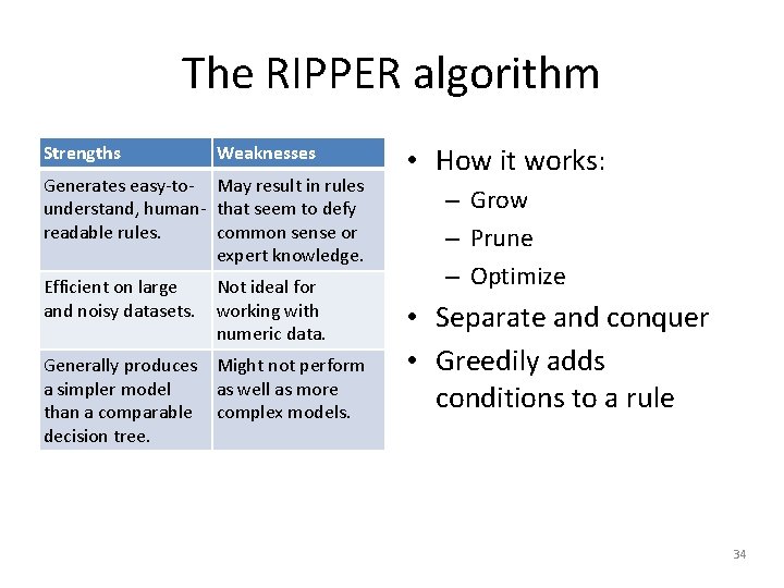
The RIPPER algorithm Strengths Weaknesses Generates easy-to- May result in rules understand, human- that seem to defy readable rules. common sense or expert knowledge. Efficient on large and noisy datasets. Not ideal for working with numeric data. Generally produces Might not perform a simpler model as well as more than a comparable complex models. decision tree. • How it works: – Grow – Prune – Optimize • Separate and conquer • Greedily adds conditions to a rule 34

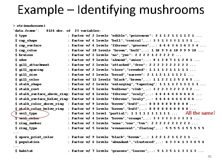
Example – Identifying mushrooms > str(mushrooms) 'data. frame': 8124 obs. of $ type : $ cap_shape : $ cap_surface : $ cap_color : $ bruises : $ odor : $ gill_attachment : $ gill_spacing : $ gill_size : $ gill_color : $ stalk_shape : $ stalk_root : $ stalk_surface_above_ring: $ stalk_surface_below_ring: $ stalk_color_above_ring : $ stalk_color_below_ring : $ veil_type : $ veil_color : $ ring_number : $ ring_type : . . . $ spore_print_color : $ population : . . . $ habitat : 23 variables: Factor w/ 2 levels "edible", "poisonous": 2 1 1 1 1 2 1. . . Factor w/ 6 levels "bell", "conical", . . : 3 3 1 3 3 3 1 1 3 1. . . Factor w/ 4 levels "fibrous", "grooves", . . : 4 4 4 3 4 3 3 4. . . Factor w/ 10 levels "brown", "buff", . . : 1 10 9 9 4 10 9 9 9 10. . . Factor w/ 2 levels "no", "yes": 2 2 1 2 2 2. . . Factor w/ 9 levels "almond", "anise", . . : 8 1 2 8 7 1 1 2 8 1. . . Factor w/ 2 levels "attached", "free": 2 2 2 2 2. . . Factor w/ 2 levels "close", "crowded": 1 1 2 1 1 1. . . Factor w/ 2 levels "broad", "narrow": 2 1 1 1 1 2 1. . . Factor w/ 12 levels "black", "brown", . . : 1 1 2 2 1 2 5 2 8 5. . . Factor w/ 2 levels "enlarging", "tapering": 1 1 2 1 1 1. . . Factor w/ 5 levels "bulbous", "club", . . : 3 2 2 3 3 2 2 2 3 2. . . Factor w/ 4 levels "fibrous", "scaly", . . : 4 4 4 4 4. . . Factor w/ 9 levels "brown", "buff", . . : 8 8 8 8 8. . . Factor w/ 1 level "partial": 1 1 1 1 1. . . Factor w/ 4 levels "brown", "orange", . . : 3 3 3 3 3. . . Factor w/ 3 levels "none", "two": 2 2 2 2 2. . . Factor w/ 5 levels "evanescent", "flaring", . . : 5 5 1 5 5 5 All the same! Factor w/ 9 levels "black", "brown", . . : 1 2 2 1 1. . . Factor w/ 6 levels "abundant", "clustered", . . : 4 3 3 4 1 3 3 4 5 4 Factor w/ 7 levels "grasses", "leaves", . . : 5 1 3 5 1 1 3 3 1 3. . . 35

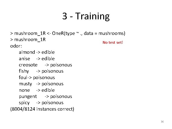
3 - Training > mushroom_1 R <- One. R(type ~. , data = mushrooms) > mushroom_1 R No test set! odor: almond -> edible anise -> edible creosote -> poisonous fishy -> poisonous foul-> poisonous musty -> poisonous none -> edible pungent -> poisonous spicy -> poisonous (8004/8124 instances correct) 36

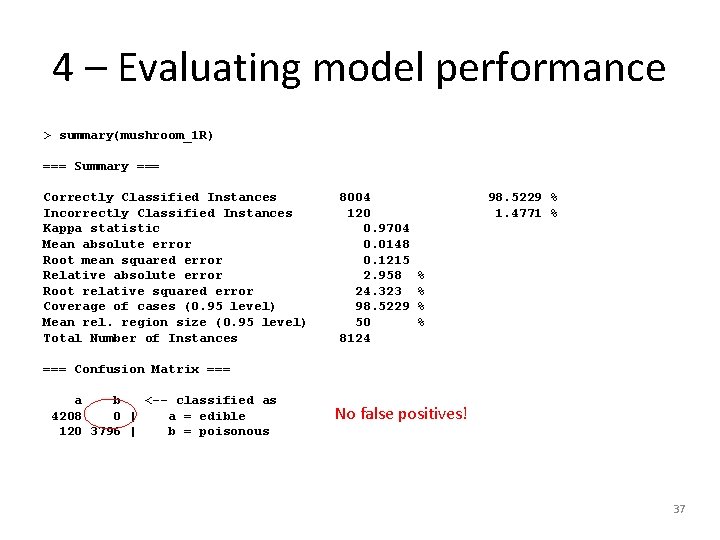
4 – Evaluating model performance > summary(mushroom_1 R) === Summary === Correctly Classified Instances Incorrectly Classified Instances Kappa statistic Mean absolute error Root mean squared error Relative absolute error Root relative squared error Coverage of cases (0. 95 level) Mean rel. region size (0. 95 level) Total Number of Instances 8004 120 0. 9704 0. 0148 0. 1215 2. 958 24. 323 98. 5229 50 8124 98. 5229 % 1. 4771 % % % === Confusion Matrix === a b <-- classified as 4208 0 | a = edible 120 3796 | b = poisonous No false positives! 37

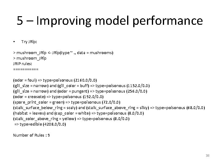
5 – Improving model performance • Try JRip: > mushroom_JRip <- JRip(type ~. , data = mushrooms) > mushroom_JRip JRIP rules: ====== (odor = foul) => type=poisonous (2160. 0/0. 0) (gill_size = narrow) and (gill_color = buff) => type=poisonous (1152. 0/0. 0) (gill_size = narrow) and (odor = pungent) => type=poisonous (256. 0/0. 0) (odor = creosote) => type=poisonous (192. 0/0. 0) (spore_print_color = green) => type=poisonous (72. 0/0. 0) (stalk_surface_below_ring = scaly) and (stalk_surface_above_ring = silky) => type=poisonous (68. 0/0. 0) (habitat = leaves) and (cap_color = white) => type=poisonous (8. 0/0. 0) (stalk_color_above_ring = yellow) => type=poisonous (8. 0/0. 0) => type=edible (4208. 0/0. 0) Number of Rules : 9 38

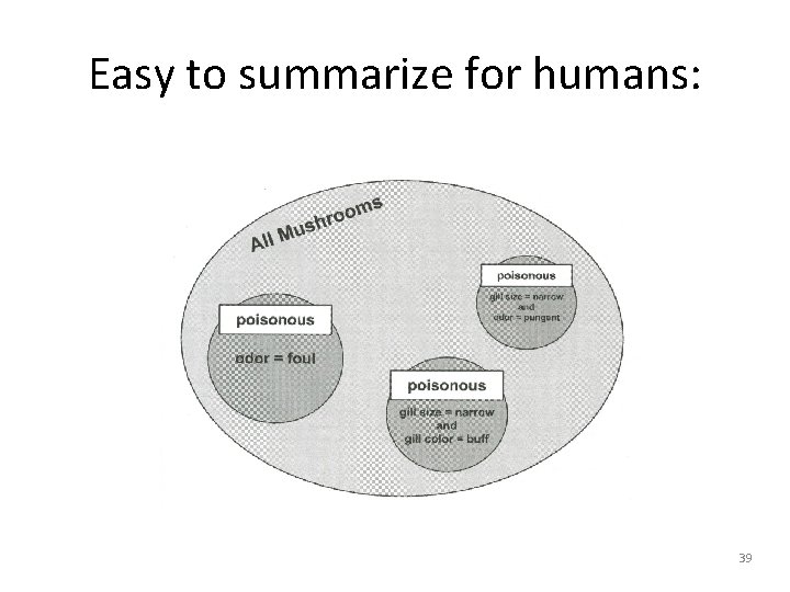
Easy to summarize for humans: 39