A 2 Level Maths Statistics 2 for Edexcel

A 2 -Level Maths: Statistics 2 for Edexcel S 2. 1 Binomial and Poisson distributions This icon indicates the slide contains activities created in Flash. These activities are not editable. For more detailed instructions, see the Getting Started presentation. 11 of of 58 58 © Boardworks Ltd 2006

Binomial distributions Contents Mean and variance of a binomial Use of binomial tables The Poisson distribution Poisson tables Mean and variance Approximating a binomial by a Poisson 22 of of 58 58 © Boardworks Ltd 2006

Special distributions Many real-life situations can be modelled using statistical distributions. Examples of the types of problem that can be addressed using these distributions include: In a board game, players needs a six before they can start. What is the probability that they haven’t started after 5 tries? What proportion of the adult population have an IQ above 120? The number of accidents on a stretch of motorway averages 1 every 2 days. How likely is it that there will be no accidents in a week? 12% of people are left-handed. What is the probability that a class of 30 people will have more than 6 left-handed people? 3 of 58 © Boardworks Ltd 2006

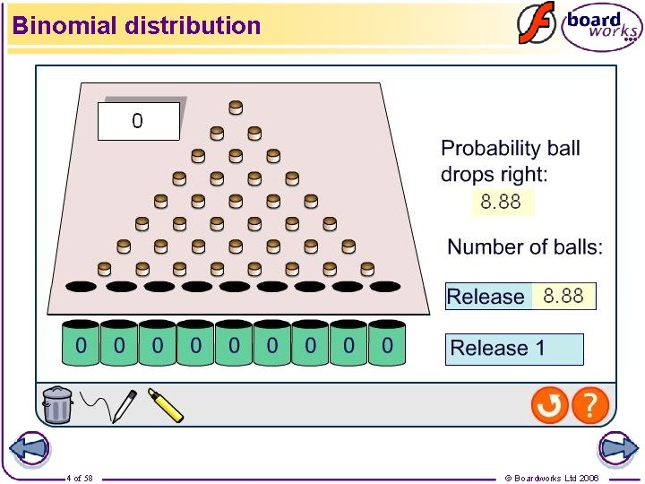
Binomial distribution 4 of 58 © Boardworks Ltd 2006

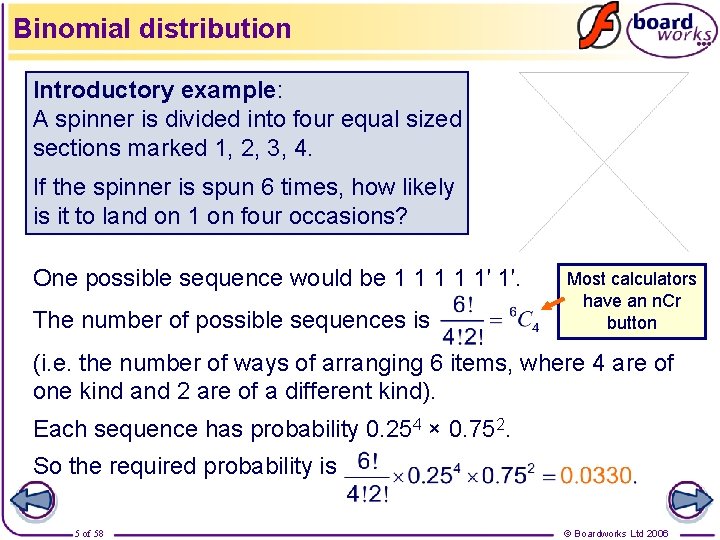
Binomial distribution Introductory example: A spinner is divided into four equal sized sections marked 1, 2, 3, 4. If the spinner is spun 6 times, how likely is it to land on 1 on four occasions? One possible sequence would be 1 1 1′ 1′. The number of possible sequences is Most calculators have an n. Cr button (i. e. the number of ways of arranging 6 items, where 4 are of one kind and 2 are of a different kind). Each sequence has probability 0. 254 × 0. 752. So the required probability is 5 of 58 © Boardworks Ltd 2006

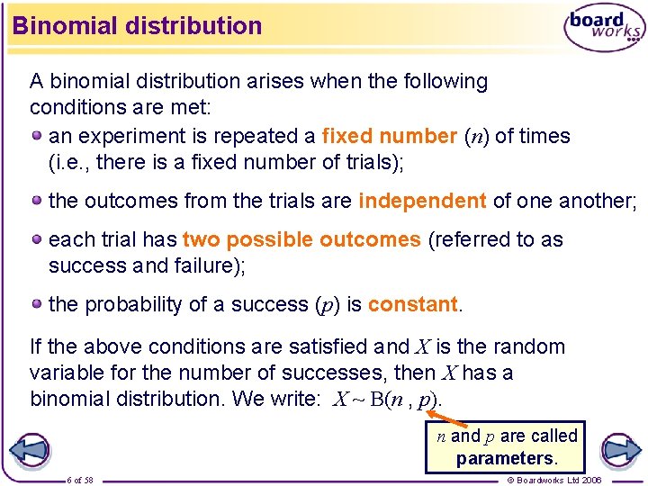
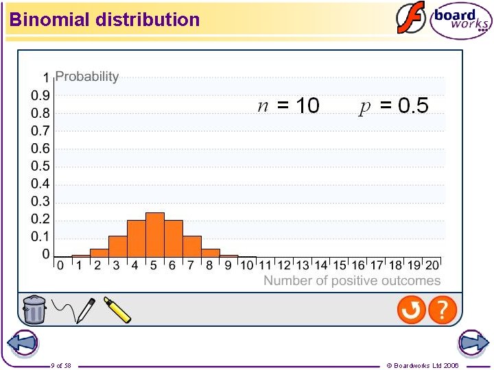
Binomial distribution A binomial distribution arises when the following conditions are met: an experiment is repeated a fixed number (n) of times (i. e. , there is a fixed number of trials); the outcomes from the trials are independent of one another; each trial has two possible outcomes (referred to as success and failure); the probability of a success (p) is constant. If the above conditions are satisfied and X is the random variable for the number of successes, then X has a binomial distribution. We write: X ~ B(n , p). n and p are called parameters. 6 of 58 © Boardworks Ltd 2006

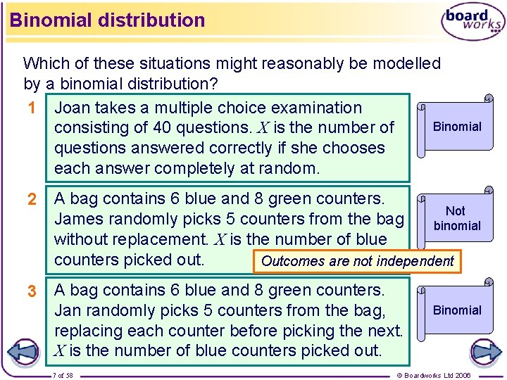
Binomial distribution Which of these situations might reasonably be modelled by a binomial distribution? 1 Joan takes a multiple choice examination Binomial consisting of 40 questions. X is the number of questions answered correctly if she chooses each answer completely at random. 2 A bag contains 6 blue and 8 green counters. Not James randomly picks 5 counters from the bag binomial without replacement. X is the number of blue counters picked out. Outcomes are not independent 3 A bag contains 6 blue and 8 green counters. Jan randomly picks 5 counters from the bag, replacing each counter before picking the next. X is the number of blue counters picked out. 7 of 58 Binomial © Boardworks Ltd 2006

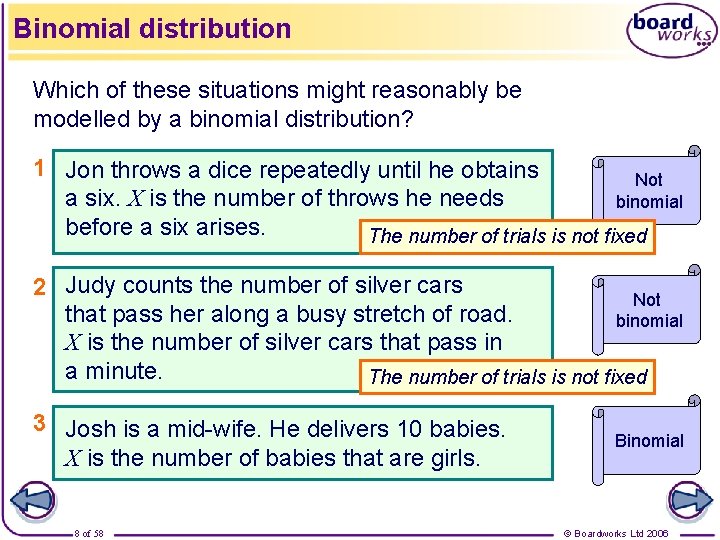
Binomial distribution Which of these situations might reasonably be modelled by a binomial distribution? 1 Jon throws a dice repeatedly until he obtains Not a six. X is the number of throws he needs binomial before a six arises. The number of trials is not fixed 2 Judy counts the number of silver cars Not that pass her along a busy stretch of road. binomial X is the number of silver cars that pass in a minute. The number of trials is not fixed 3 Josh is a mid-wife. He delivers 10 babies. X is the number of babies that are girls. 8 of 58 Binomial © Boardworks Ltd 2006

Binomial distribution 9 of 58 © Boardworks Ltd 2006

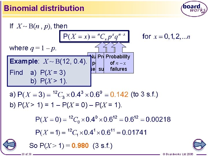
Binomial distribution If X ~ B(n , p), then where q = 1 – p. Example: X ~ B(12, 0. 4). Find a) P(X = 3) b) P(X > 1). Number Probability of ofof x n–x possible sequences successes failures a) (to 3 s. f. ) b) P(X > 1) = 1 – P(X = 0) – P(X = 1). So P(X > 1) = 0. 980 (3 s. f. ) 10 of 58 © Boardworks Ltd 2006

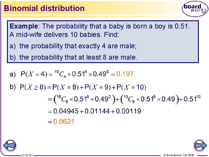
Binomial distribution Example: The probability that a baby is born a boy is 0. 51. A mid-wife delivers 10 babies. Find: a) the probability that exactly 4 are male; b) the probability that at least 8 are male. a) b) 11 of 58 © Boardworks Ltd 2006

Mean and variance of a binomial Binomial distributions Contents Mean and variance of a binomial Use of binomial tables The Poisson distribution Poisson tables Mean and variance Approximating a binomial by a Poisson 12 of 58 © Boardworks Ltd 2006

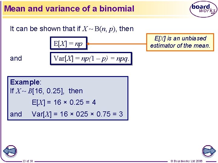
Mean and variance of a binomial It can be shown that if X ~ B(n, p), then E[X] = np and E[X] is an unbiased estimator of the mean. Var[X] = np(1 – p) = npq. Example: If X ~ B[16, 0. 25], then E[X] = 16 × 0. 25 = 4 and Var[X] = 16 × 025 × 0. 75 = 3 13 of 58 © Boardworks Ltd 2006

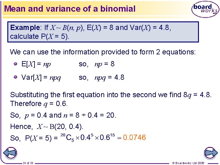
Mean and variance of a binomial Example: If X ~ B(n, p), E(X) = 8 and Var(X) = 4. 8, calculate P(X = 5). We can use the information provided to form 2 equations: E[X] = np so, np = 8 Var[X] = npq so, npq = 4. 8 Substituting the first equation into the second we find 8 q = 4. 8. Therefore q = 0. 6. So, p = 0. 4 and n = 8 ÷ 0. 4 = 20. Hence, X ~ B(20, 0. 4). So, P(X = 5) = 14 of 58 © Boardworks Ltd 2006

Use of binomial tables Binomial distributions Contents Mean and variance of a binomial Use of binomial tables The Poisson distribution Poisson tables Mean and variance Approximating a binomial by a Poisson 15 of 58 © Boardworks Ltd 2006

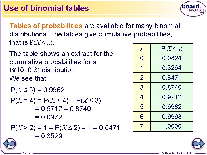
Use of binomial tables Tables of probabilities are available for many binomial distributions. The tables give cumulative probabilities, that is P(X ≤ x). x P(X ≤ x) 0 0. 0824 1 0. 3294 2 0. 6471 P(X ≤ 5) = 0. 9962 3 0. 8740 P(X = 4) = P(X ≤ 4) – P(X ≤ 3) = 0. 9712 – 0. 8740 = 0. 0972 4 0. 9712 5 0. 9962 6 0. 9998 P(X > 2) = 1 – P(X ≤ 2) = 1 – 0. 6471 = 0. 3529 7 1. 0000 The table shows an extract for the cumulative probabilities for a B(10, 0. 3) distribution. We see that: 16 of 58 © Boardworks Ltd 2006

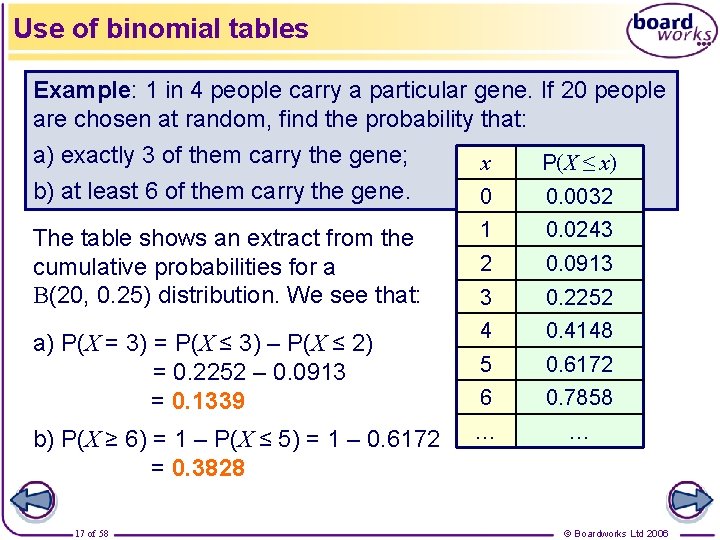
Use of binomial tables Example: 1 in 4 people carry a particular gene. If 20 people are chosen at random, find the probability that: a) exactly 3 of them carry the gene; x P(X ≤ x) b) at least 6 of them carry the gene. 0 0. 0032 The table shows an extract from the cumulative probabilities for a B(20, 0. 25) distribution. We see that: a) P(X = 3) = P(X ≤ 3) – P(X ≤ 2) = 0. 2252 – 0. 0913 = 0. 1339 b) P(X ≥ 6) = 1 – P(X ≤ 5) = 1 – 0. 6172 = 0. 3828 17 of 58 1 0. 0243 2 0. 0913 3 0. 2252 4 0. 4148 5 0. 6172 6 0. 7858 … … © Boardworks Ltd 2006

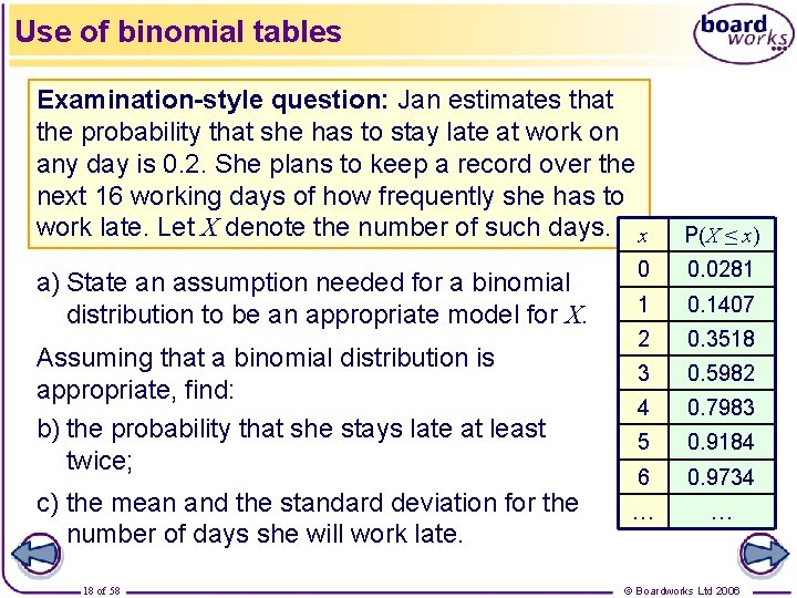
Use of binomial tables Examination-style question: Jan estimates that the probability that she has to stay late at work on any day is 0. 2. She plans to keep a record over the next 16 working days of how frequently she has to work late. Let X denote the number of such days. x P(X ≤ x) 0 0. 0281 1 0. 1407 2 0. 3518 3 0. 5982 4 0. 7983 5 0. 9184 6 0. 9734 … … a) State an assumption needed for a binomial distribution to be an appropriate model for X. Assuming that a binomial distribution is appropriate, find: b) the probability that she stays late at least twice; c) the mean and the standard deviation for the number of days she will work late. 18 of 58 © Boardworks Ltd 2006

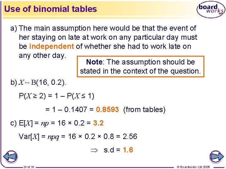
Use of binomial tables a) The main assumption here would be that the event of her staying on late at work on any particular day must be independent of whether she had to work late on any other day. Note: The assumption should be stated in the context of the question. b) X ~ B(16, 0. 2). P(X ≥ 2) = 1 – P(X ≤ 1) = 1 – 0. 1407 = 0. 8593 (from tables) c) E[X] = np = 16 × 0. 2 = 3. 2 Var[X] = npq = 16 × 0. 2 × 0. 8 = 2. 56 s. d = 1. 6 19 of 58 © Boardworks Ltd 2006

The Poisson distribution Binomial distributions Contents Mean and variance of a binomial Use of binomial tables The Poisson distribution Poisson tables Mean and variance Approximating a binomial by a Poisson 20 of 58 © Boardworks Ltd 2006

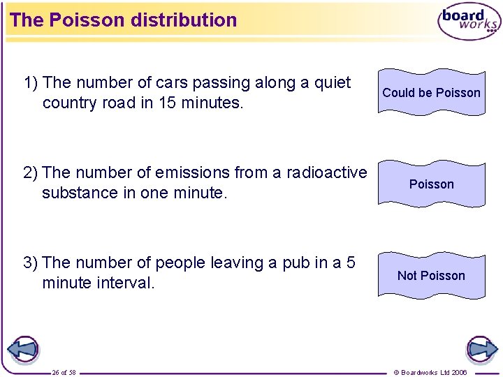
Introduction We are sometimes interested in the number of times an event occurs in a period of space or time: 1) Sam counts the number of cars travelling past her on a quiet country road. X represents the number of cars passing her in 15 minutes. 2) Xiu uses a Geiger counter to record the number of particles emitted by a radioactive substance. X is the number of emissions in one minute. 3) Scott counts the number of people leaving a pub. X is the number of people leaving in a 5 minute interval. 21 of 58 © Boardworks Ltd 2006

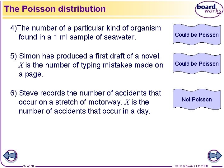
Introduction 4) Selina is taking samples of sea water. X is the number of a particular kind of organism that she finds in a 1 ml sample of water. 5) Ankur has produced a first draft of a novel. X is the number of typing mistakes made on a page. 6) Steve records the number of accidents that occur on a stretch of motorway. X is the number of accidents that occur in a day. 22 of 58 © Boardworks Ltd 2006

The Poisson distribution In each of these situations, the random variable X counts the number of times an event occurs in a given amount of space or time. X takes the values 0, 1, 2, 3, …. The Poisson distribution is a model that can sometimes be used for count data. The distribution is named after the French mathematician and scientist Siméon Denis Poisson (17811840). The Poisson distribution has a number of conditions. 23 of 58 © Boardworks Ltd 2006

Conditions for a Poisson distribution A random variable, X, which counts the number of times an event occurs in a given unit of space or time will have a Poisson distribution if: the events occur independently of each other and at random; the events occur at a constant rate (in the sense that the number of events occurring in a given interval is directly proportional to the length of that interval); the events occur singly (that is, one at a time). 24 of 58 © Boardworks Ltd 2006

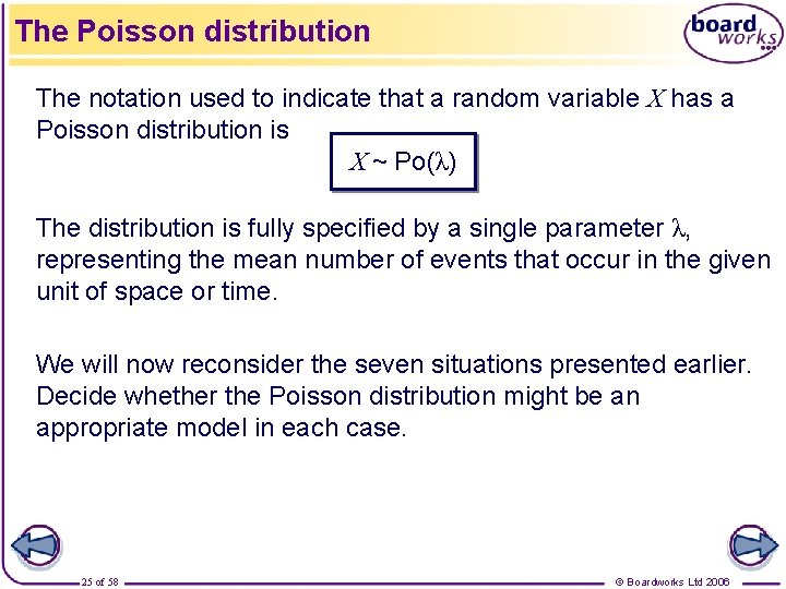
The Poisson distribution The notation used to indicate that a random variable X has a Poisson distribution is X ~ Po(λ) The distribution is fully specified by a single parameter λ, representing the mean number of events that occur in the given unit of space or time. We will now reconsider the seven situations presented earlier. Decide whether the Poisson distribution might be an appropriate model in each case. 25 of 58 © Boardworks Ltd 2006

The Poisson distribution 1) The number of cars passing along a quiet country road in 15 minutes. 2) The number of emissions from a radioactive substance in one minute. 3) The number of people leaving a pub in a 5 minute interval. 26 of 58 Could be Poisson Not Poisson © Boardworks Ltd 2006

The Poisson distribution 4)The number of a particular kind of organism found in a 1 ml sample of seawater. Could be Poisson 5) Simon has produced a first draft of a novel. X is the number of typing mistakes made on a page. Could be Poisson 6) Steve records the number of accidents that occur on a stretch of motorway. X is the number of accidents that occur in a day. Not Poisson 27 of 58 © Boardworks Ltd 2006

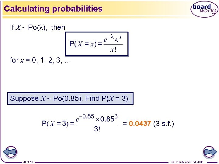
Calculating probabilities If X ~ Po(λ), then for x = 0, 1, 2, 3, … Suppose X ~ Po(0. 85). Find P(X = 3). = 0. 0437 (3 s. f. ) 28 of 58 © Boardworks Ltd 2006

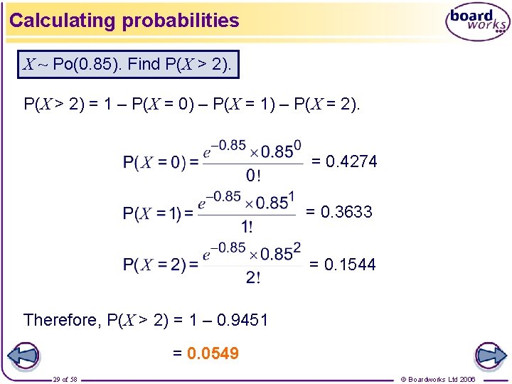
Calculating probabilities X ~ Po(0. 85). Find P(X > 2) = 1 – P(X = 0) – P(X = 1) – P(X = 2). = 0. 4274 = 0. 3633 = 0. 1544 Therefore, P(X > 2) = 1 – 0. 9451 = 0. 0549 29 of 58 © Boardworks Ltd 2006

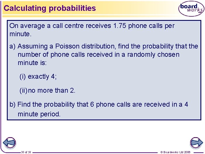
Calculating probabilities On average a call centre receives 1. 75 phone calls per minute. a) Assuming a Poisson distribution, find the probability that the number of phone calls received in a randomly chosen minute is: (i) exactly 4; (ii) no more than 2. b) Find the probability that 6 phone calls are received in a 4 minute period. 30 of 58 © Boardworks Ltd 2006

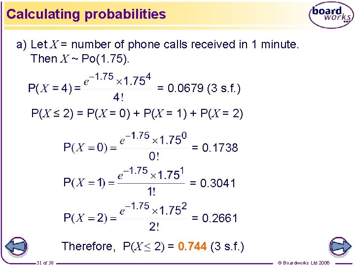
Calculating probabilities a) Let X = number of phone calls received in 1 minute. Then X ~ Po(1. 75). = 0. 0679 (3 s. f. ) P(X ≤ 2) = P(X = 0) + P(X = 1) + P(X = 2) = 0. 1738 = 0. 3041 = 0. 2661 Therefore, P(X ≤ 2) = 0. 744 (3 s. f. ) 31 of 58 © Boardworks Ltd 2006

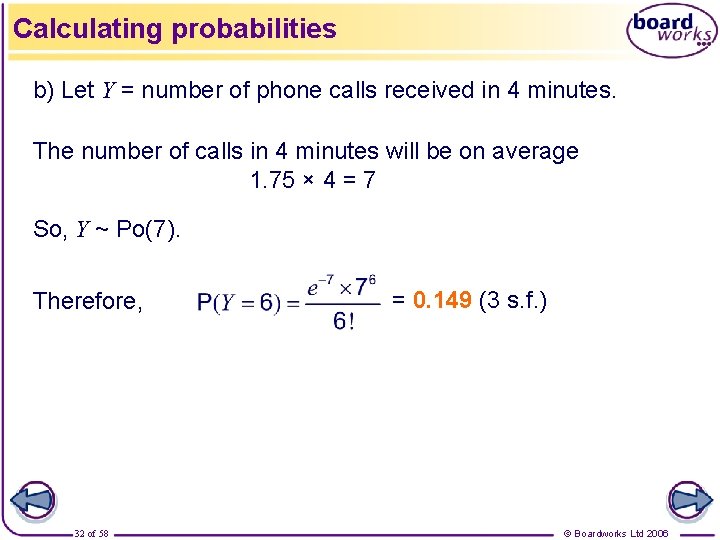
Calculating probabilities b) Let Y = number of phone calls received in 4 minutes. The number of calls in 4 minutes will be on average 1. 75 × 4 = 7 So, Y ~ Po(7). Therefore, 32 of 58 = 0. 149 (3 s. f. ) © Boardworks Ltd 2006

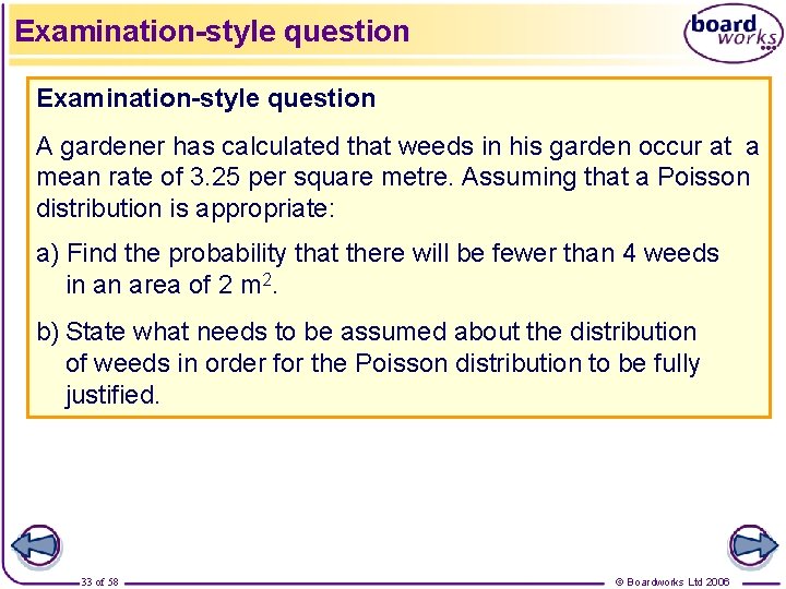
Examination-style question A gardener has calculated that weeds in his garden occur at a mean rate of 3. 25 per square metre. Assuming that a Poisson distribution is appropriate: a) Find the probability that there will be fewer than 4 weeds in an area of 2 m 2. b) State what needs to be assumed about the distribution of weeds in order for the Poisson distribution to be fully justified. 33 of 58 © Boardworks Ltd 2006

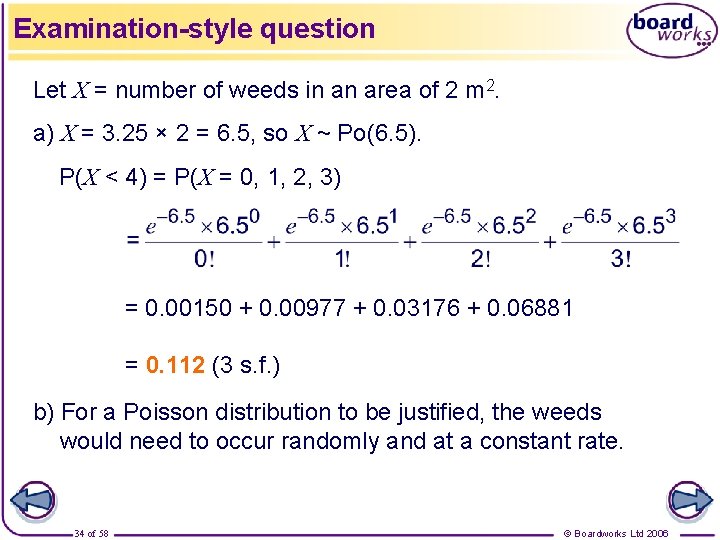
Examination-style question Let X = number of weeds in an area of 2 m 2. a) X = 3. 25 × 2 = 6. 5, so X ~ Po(6. 5). P(X < 4) = P(X = 0, 1, 2, 3) = 0. 00150 + 0. 00977 + 0. 03176 + 0. 06881 = 0. 112 (3 s. f. ) b) For a Poisson distribution to be justified, the weeds would need to occur randomly and at a constant rate. 34 of 58 © Boardworks Ltd 2006

Poisson tables Binomial distributions Contents Mean and variance of a binomial Use of binomial tables The Poisson distribution Poisson tables Mean and variance Approximating a binomial by a Poisson 35 of 58 © Boardworks Ltd 2006

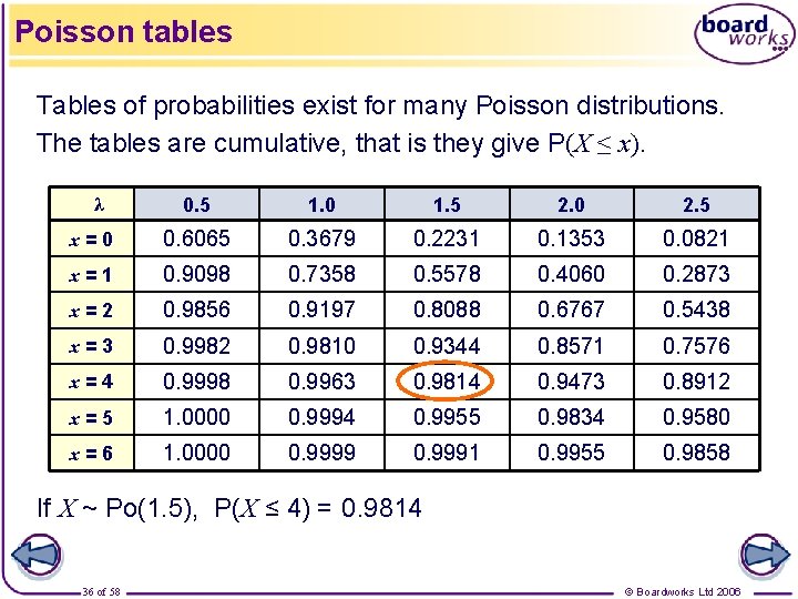
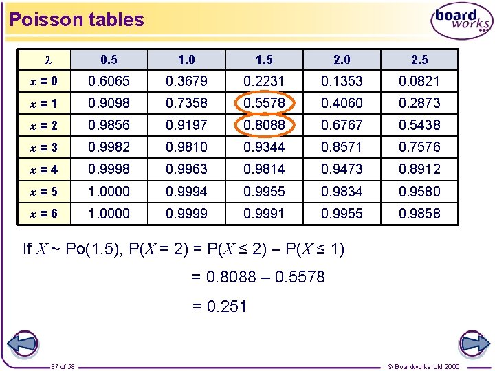
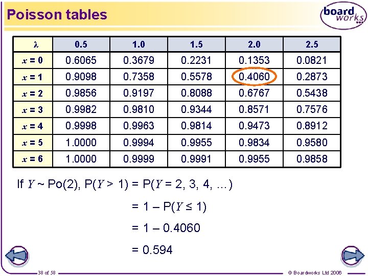
Poisson tables Tables of probabilities exist for many Poisson distributions. The tables are cumulative, that is they give P(X ≤ x). 0. 5 1. 0 1. 5 2. 0 2. 5 x=0 0. 6065 0. 3679 0. 2231 0. 1353 0. 0821 x=1 0. 9098 0. 7358 0. 5578 0. 4060 0. 2873 x=2 0. 9856 0. 9197 0. 8088 0. 6767 0. 5438 x=3 0. 9982 0. 9810 0. 9344 0. 8571 0. 7576 x=4 0. 9998 0. 9963 0. 9814 0. 9473 0. 8912 x=5 1. 0000 0. 9994 0. 9955 0. 9834 0. 9580 x=6 1. 0000 0. 9999 0. 9991 0. 9955 0. 9858 λ If X ~ Po(1. 5), P(X ≤ 4) = 0. 9814 36 of 58 © Boardworks Ltd 2006

Poisson tables 0. 5 1. 0 1. 5 2. 0 2. 5 x=0 0. 6065 0. 3679 0. 2231 0. 1353 0. 0821 x=1 0. 9098 0. 7358 0. 5578 0. 4060 0. 2873 x=2 0. 9856 0. 9197 0. 8088 0. 6767 0. 5438 x=3 0. 9982 0. 9810 0. 9344 0. 8571 0. 7576 x=4 0. 9998 0. 9963 0. 9814 0. 9473 0. 8912 x=5 1. 0000 0. 9994 0. 9955 0. 9834 0. 9580 x=6 1. 0000 0. 9999 0. 9991 0. 9955 0. 9858 λ If X ~ Po(1. 5), P(X = 2) = P(X ≤ 2) – P(X ≤ 1) = 0. 8088 – 0. 5578 = 0. 251 37 of 58 © Boardworks Ltd 2006

Poisson tables 0. 5 1. 0 1. 5 2. 0 2. 5 x=0 0. 6065 0. 3679 0. 2231 0. 1353 0. 0821 x=1 0. 9098 0. 7358 0. 5578 0. 4060 0. 2873 x=2 0. 9856 0. 9197 0. 8088 0. 6767 0. 5438 x=3 0. 9982 0. 9810 0. 9344 0. 8571 0. 7576 x=4 0. 9998 0. 9963 0. 9814 0. 9473 0. 8912 x=5 1. 0000 0. 9994 0. 9955 0. 9834 0. 9580 x=6 1. 0000 0. 9999 0. 9991 0. 9955 0. 9858 λ If Y ~ Po(2), P(Y > 1) = P(Y = 2, 3, 4, …) = 1 – P(Y ≤ 1) = 1 – 0. 4060 = 0. 594 38 of 58 © Boardworks Ltd 2006

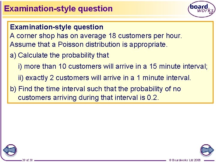
Examination-style question A corner shop has on average 18 customers per hour. Assume that a Poisson distribution is appropriate. a) Calculate the probability that i) more than 10 customers will arrive in a 15 minute interval; ii) exactly 2 customers will arrive in a 1 minute interval. b) Find the time interval such that the probability of no customers arriving during that interval is 0. 2. 39 of 58 © Boardworks Ltd 2006

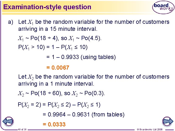
Examination-style question a) Let X 1 be the random variable for the number of customers arriving in a 15 minute interval. X 1 ~ Po(18 ÷ 4), so X 1 ~ Po(4. 5). P(X 1 > 10) = 1 – P(X 1 ≤ 10) = 1 – 0. 9933 (using tables) = 0. 0067 Let X 2 be the random variable for the number of customers arriving in a 1 minute interval. X 2 ~ Po(18 ÷ 60), so X 2 ~ Po(0. 3). P(X 2 = 2) = P(X 2 ≤ 2) – P(X 2 ≤ 1) = 0. 9964 – 0. 9631 (from tables) = 0. 0333 40 of 58 © Boardworks Ltd 2006

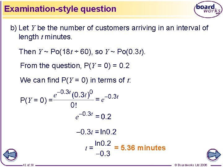
Examination-style question b) Let Y be the number of customers arriving in an interval of length t minutes. Then Y ~ Po(18 t ÷ 60), so Y ~ Po(0. 3 t). From the question, P(Y = 0) = 0. 2 We can find P(Y = 0) in terms of t : P(Y = 0) = = 5. 36 minutes 41 of 58 © Boardworks Ltd 2006

Mean and variance Binomial distributions Contents Mean and variance of a binomial Use of binomial tables The Poisson distribution Poisson tables Mean and variance Approximating a binomial by a Poisson 42 of 58 © Boardworks Ltd 2006

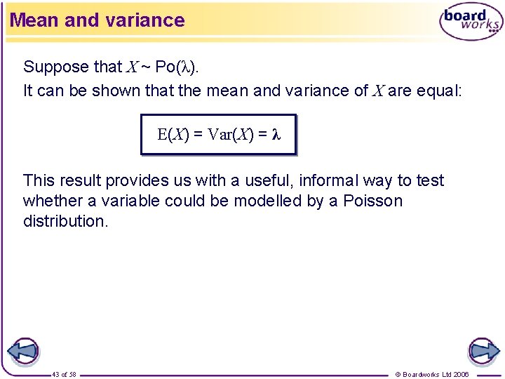
Mean and variance Suppose that X ~ Po(λ). It can be shown that the mean and variance of X are equal: E(X) = Var(X) = λ This result provides us with a useful, informal way to test whether a variable could be modelled by a Poisson distribution. 43 of 58 © Boardworks Ltd 2006

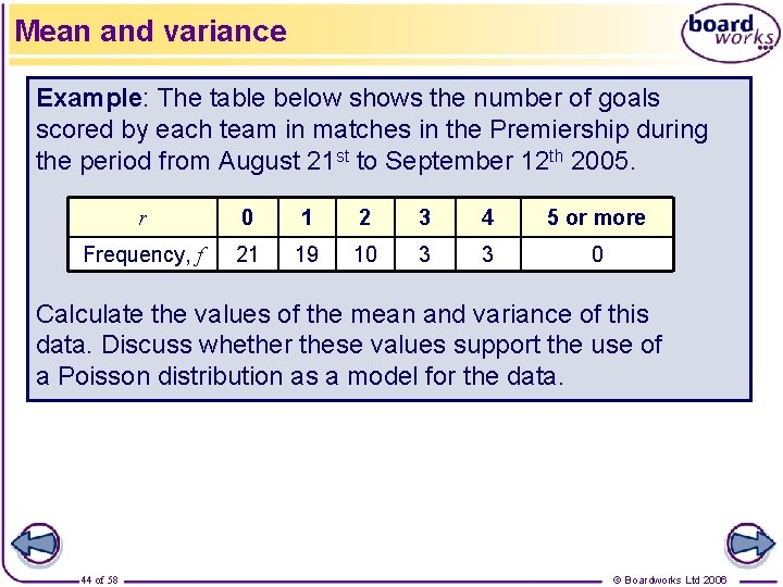
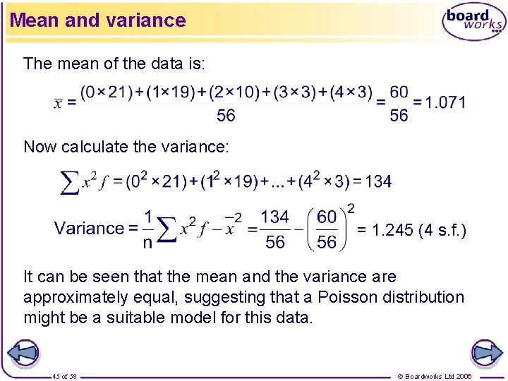
Mean and variance Example: The table below shows the number of goals scored by each team in matches in the Premiership during the period from August 21 st to September 12 th 2005. r 0 1 2 3 4 5 or more Frequency, f 21 19 10 3 3 0 Calculate the values of the mean and variance of this data. Discuss whether these values support the use of a Poisson distribution as a model for the data. 44 of 58 © Boardworks Ltd 2006

Mean and variance The mean of the data is: Now calculate the variance: = 1. 245 (4 s. f. ) It can be seen that the mean and the variance are approximately equal, suggesting that a Poisson distribution might be a suitable model for this data. 45 of 58 © Boardworks Ltd 2006

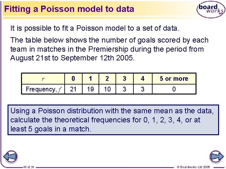
Fitting a Poisson model to data It is possible to fit a Poisson model to a set of data. The table below shows the number of goals scored by each team in matches in the Premiership during the period from August 21 st to September 12 th 2005. r 0 1 2 3 4 5 or more Frequency, f 21 19 10 3 3 0 Using a Poisson distribution with the same mean as the data, calculate theoretical frequencies for 0, 1, 2, 3, 4, or at least 5 goals in a match. 46 of 58 © Boardworks Ltd 2006

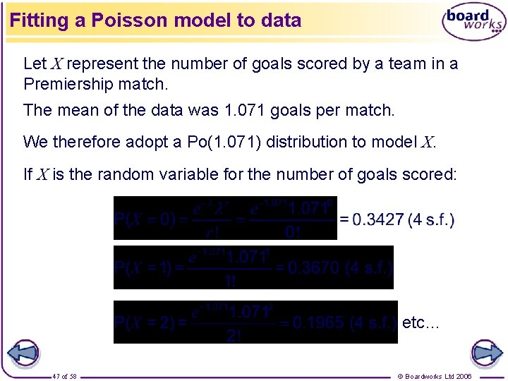
Fitting a Poisson model to data Let X represent the number of goals scored by a team in a Premiership match. The mean of the data was 1. 071 goals per match. We therefore adopt a Po(1. 071) distribution to model X. If X is the random variable for the number of goals scored: etc… 47 of 58 © Boardworks Ltd 2006

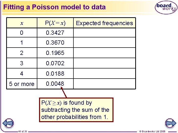
Fitting a Poisson model to data x P(X = x) 0 0. 3427 1 0. 3670 2 0. 1965 3 0. 0702 4 0. 0188 5 or more 0. 0048 Expected frequencies P(X ≥ x) is found by subtracting the sum of the other probabilities from 1. 48 of 58 © Boardworks Ltd 2006

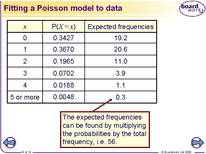
Fitting a Poisson model to data x P(X = x) Expected frequencies 0 0. 3427 19. 2 1 0. 3670 20. 6 2 0. 1965 11. 0 3 0. 0702 3. 9 4 0. 0188 1. 1 5 or more 0. 0048 0. 3 The expected frequencies can be found by multiplying the probabilities by the total frequency, i. e. 56. 49 of 58 © Boardworks Ltd 2006

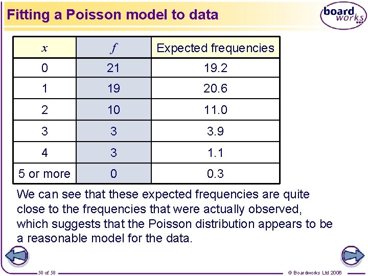
Fitting a Poisson model to data x f Expected frequencies 0 21 19. 2 1 19 20. 6 2 10 11. 0 3 3 3. 9 4 3 1. 1 5 or more 0 0. 3 We can see that these expected frequencies are quite close to the frequencies that were actually observed, which suggests that the Poisson distribution appears to be a reasonable model for the data. 50 of 58 © Boardworks Ltd 2006

Approximating a binomial by a Poisson Binomial distributions Contents Mean and variance of a binomial Use of binomial tables The Poisson distribution Poisson tables Mean and variance Approximating a binomial by a Poisson 51 of 58 © Boardworks Ltd 2006

Approximating a binomial by a Poisson 52 of 58 © Boardworks Ltd 2006

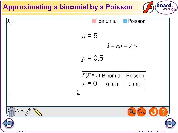
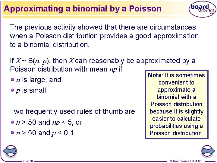
Approximating a binomial by a Poisson The previous activity showed that there are circumstances when a Poisson distribution provides a good approximation to a binomial distribution. If X ~ B(n, p), then X can reasonably be approximated by a Poisson distribution with mean np if Note: It is sometimes n is large, and convenient to approximate a p is small. Two frequently used rules of thumb are n > 50 and np < 5, or n > 50 and p < 0. 1. 53 of 58 binomial with a Poisson distribution because it is slightly easier to calculate probabilities using a Poisson distribution. © Boardworks Ltd 2006

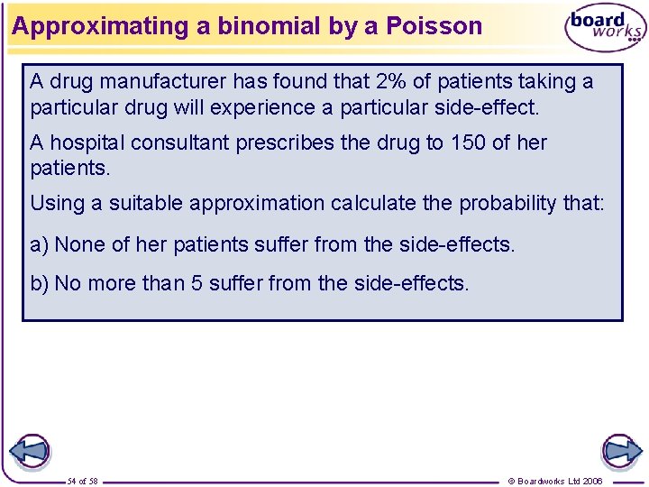
Approximating a binomial by a Poisson A drug manufacturer has found that 2% of patients taking a particular drug will experience a particular side-effect. A hospital consultant prescribes the drug to 150 of her patients. Using a suitable approximation calculate the probability that: a) None of her patients suffer from the side-effects. b) No more than 5 suffer from the side-effects. 54 of 58 © Boardworks Ltd 2006

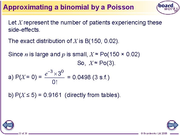
Approximating a binomial by a Poisson Let X represent the number of patients experiencing these side-effects. The exact distribution of X is B(150, 0. 02). Since n is large and p is small, X ≈ Po(150 × 0. 02) So, X ≈ Po(3). a) P(X = 0) = = 0. 0498 (3 s. f. ) b) P(X ≤ 5) = 0. 9161 (directly from tables). 55 of 58 © Boardworks Ltd 2006

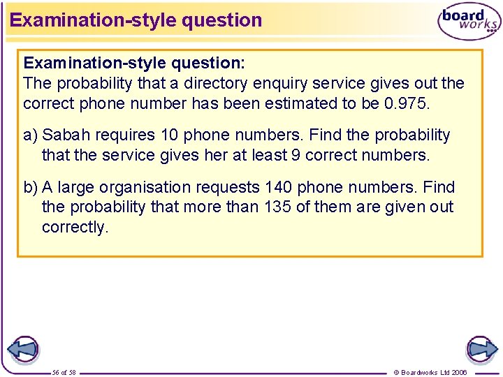
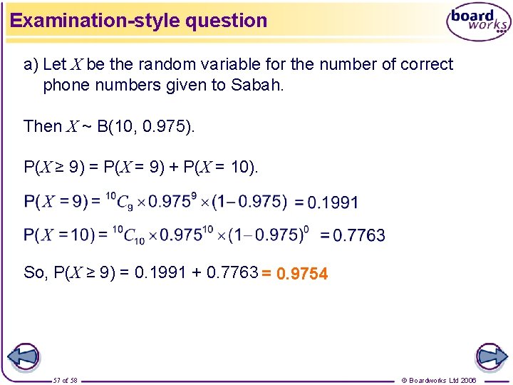
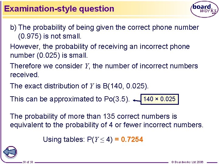
Examination-style question: The probability that a directory enquiry service gives out the correct phone number has been estimated to be 0. 975. a) Sabah requires 10 phone numbers. Find the probability that the service gives her at least 9 correct numbers. b) A large organisation requests 140 phone numbers. Find the probability that more than 135 of them are given out correctly. 56 of 58 © Boardworks Ltd 2006

Examination-style question a) Let X be the random variable for the number of correct phone numbers given to Sabah. Then X ~ B(10, 0. 975). P(X ≥ 9) = P(X = 9) + P(X = 10). So, P(X ≥ 9) = 0. 1991 + 0. 7763 = 0. 9754 57 of 58 © Boardworks Ltd 2006

Examination-style question b) The probability of being given the correct phone number (0. 975) is not small. However, the probability of receiving an incorrect phone number (0. 025) is small. Therefore we consider Y, the number of incorrect numbers received. The exact distribution of Y is B(140, 0. 025). This can be approximated to Po(3. 5). 140 × 0. 025 The probability of more than 135 correct numbers is equivalent to the probability of 4 or fewer incorrect numbers. Using tables: P(Y ≤ 4) = 0. 7254 58 of 58 © Boardworks Ltd 2006