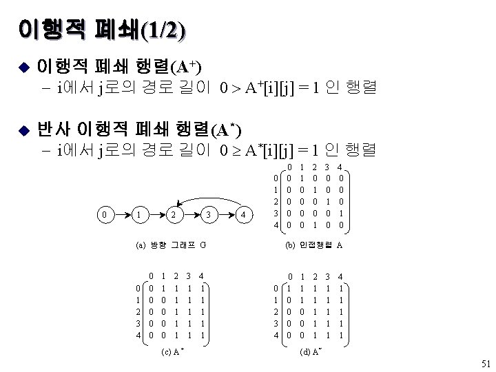
99 ADT Graph objects functions for all graph

 ADT Graph objects: 공집합이 아닌 정점의 집합과 무방향 간선의 집합으로")
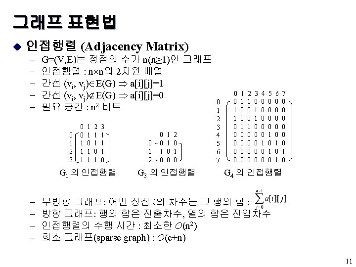
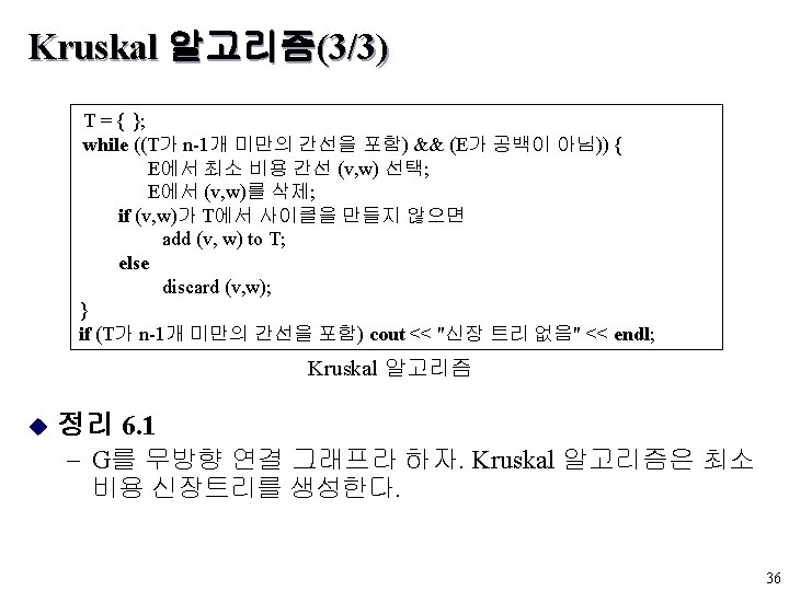
그래프 추상 데이타 타입(9/9) ADT Graph objects: 공집합이 아닌 정점의 집합과 무방향 간선의 집합으로 각 간선은 정점의 쌍이다. functions: for all graph ∈ Graph, v, v 1, and v 2 ∈ Vertices Graph Create() : : = return an empty graph Graph Insert. Vertex(graph, v) : : = return a graph with v inserted v has no incident edges Graph Insert. Edge(graph, v 1, v 2) : : = return a graph with a new edge between v 1 and v 2 Graph Delete. Vertex(graph, v) : : = return a graph in which v and all edges incident to it are removed Graph Delete. Edge(graph, v 1, v 2) : : = return a graph in which the edge(v 1, v 2) is removed Leave the incident nodes in the graph Boolean Is. Empty(graph) : : = if(graph = = empty graph) return TRUE else return FALSE List Adjacent(graph, v) : : = return a list of all vertices that are adjacent to v < 그래프 추상 데이타 타입 > 10
![인접리스트(2/4) adj. Lists [0] [1] [2] [3] data link 3 1 2 0 2](http://slidetodoc.com/presentation_image/1fe3a5588cb09a980ced0c2e6ca8990b/image-13.jpg "인접리스트(2/4) adj. Lists [0] [1] [2] [3] data link 3 1 2 0 2")
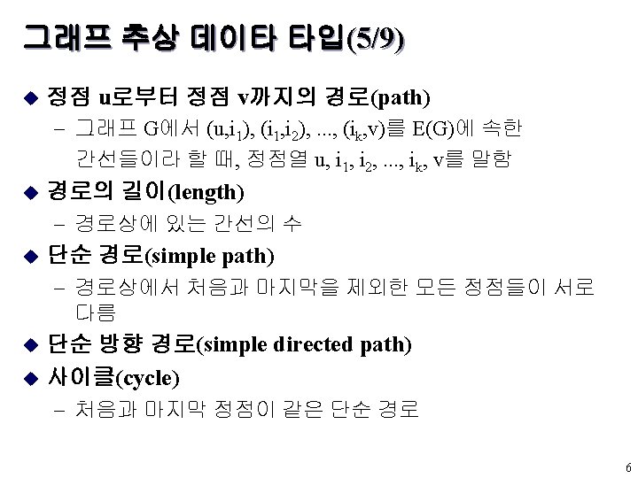
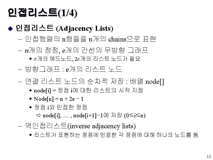
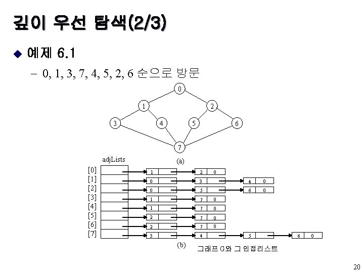
인접리스트(2/4) adj. Lists [0] [1] [2] [3] data link 3 1 2 0 2 3 0 0 1 3 0 0 0 1 2 0 G 1 인접 리스트 adj. Lists [0] [1] [2] 1 0 2 0 0 0 G 3 인접 리스트 adj. Lists [0] [1] [2] [3] [4] [5] [6] [7] 2 1 0 3 0 0 0 3 0 1 2 0 6 4 0 5 7 0 5 6 0 0 G 4 인접 리스트 ( 13
![인접리스트(3/4) int nodes[n + 2*e +1]; 0 1 2 3 4 5 6 7](http://slidetodoc.com/presentation_image/1fe3a5588cb09a980ced0c2e6ca8990b/image-14.jpg "인접리스트(3/4) int nodes[n + 2*e +1]; 0 1 2 3 4 5 6 7")
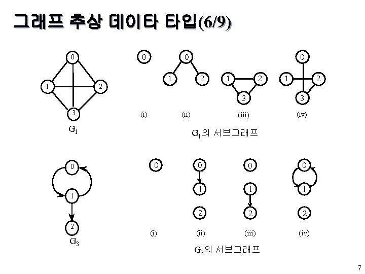
인접리스트(3/4) int nodes[n + 2*e +1]; 0 1 2 3 4 5 6 7 8 9 10 11 12 13 14 15 16 17 18 19 20 21 22 그래프 G 4의 순차 표현 G 3의 역인접리스트 14
 간선(u, v)는 두 개의 엔트리로 표현 : u를 위한 리스트, v를")
인접다중리스트 (Adjacency Multilists) 간선(u, v)는 두 개의 엔트리로 표현 : u를 위한 리스트, v를 위한 리스트에 나타남 u 새로운 노드 구조 u m vertex 1 vertex 2 list 1 list 2 adj. Nodes [0] N 0 0 1 N 3 edge (0, 1) [1] N 1 0 2 N 3 edge (0, 2) [2] N 2 0 3 0 N 4 edge (0, 3) [3] N 3 1 2 N 4 N 5 edge (1, 2) N 4 1 3 0 N 5 edge (1, 3) N 5 2 3 0 0 edge (2, 3) The lists are vertex 0: vertex 1: vertex 2: vertex 3: N 0 → N 1 → N 2 N 0 → N 3 → N 4 N 1 → N 3 → N 5 N 2 → N 4 → N 5 G 1에 대한 인접 다중리스트 16
![깊이 우선 탐색(1/3) #define FALSE 0 #define TRUE 1 short int visited[MAX_VERTICES]; void dfs](http://slidetodoc.com/presentation_image/1fe3a5588cb09a980ced0c2e6ca8990b/image-19.jpg "깊이 우선 탐색(1/3) #define FALSE 0 #define TRUE 1 short int visited[MAX_VERTICES]; void dfs")
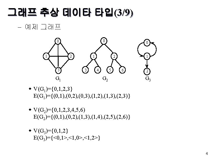
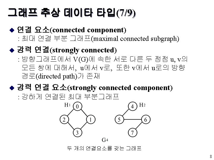
깊이 우선 탐색(1/3) #define FALSE 0 #define TRUE 1 short int visited[MAX_VERTICES]; void dfs (int v) {/* 그래프의 정점 v에서 시작하는 깊이 우선 탐색 */ node. Pointer w; visited[v] = TRUE; printf(“%5 d”, v); for (w = graph[v]; w; w = w → link) if (!visited [w→vertex]) dfs (w→vertex); } 깊이-우선 탐색 19
 void bfs(int v) {/* 정점 v에서 시작하는 너비 우선 탐색. 전역배열")
너비 우선 탐색(2/2) void bfs(int v) {/* 정점 v에서 시작하는 너비 우선 탐색. 전역배열 visited는 0으로 초기화됨} node_pointer w; queue_pointer front, rear; front = rear = NULL; /* 큐의 초기화 */ printf(“%5 d”, v); visited[v] = TRUE; addq(&front, &rear, v); while (front){ v = deleteq(&front); for (w=graph[v]; w; w=w→link) if (!visited[w→vertex]) { printf(“%5 d”, w→vertex); addq(&front, &rear, w→vertex); visited[w→vertex] = TRUE; } } } u BFS의 분석 - 전체 시간 O(n 2) - 인접 리스트 표현 : 전체 비용 O(e) 23
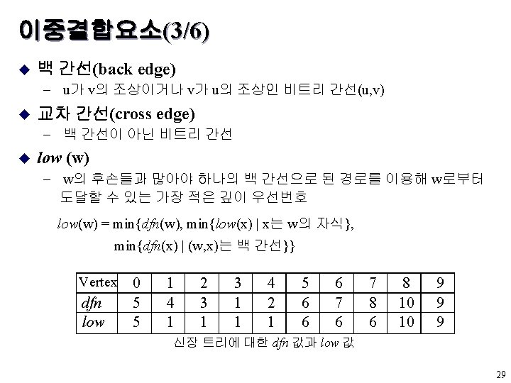
 #define MIN 2(x, y) ((x) < (y) ? (x) : (y)) short int")
이중결합요소(4/6) #define MIN 2(x, y) ((x) < (y) ? (x) : (y)) short int dfn[MAX_VERTICES]; short int low[MAX_VERTICES]; int num; void dfnlow (int u, int v) /* compute dfn and low while performing a dfs search beginning at vertex u, v is the parent of u (if any) */ node. Pointer ptr; int w; dfn[u] = low[u] = num++; for (ptr = graph[u]; ptr = ptr→link) { w = ptr → vertex; if (dfn[w] <0) { /* w is an unvisited vertex */ dfnlow(w, u); low[u] = MIN 2(low[u], low[w]); } else if (w != v) low[u] = MIN 2(low[u], dfn[w]); } } Dfn 과 low 의 계산 30
![이중결합요소(5/6) void init(void) { int i; for (i=0; i<n; i++) { visited[i] = FALSE;](http://slidetodoc.com/presentation_image/1fe3a5588cb09a980ced0c2e6ca8990b/image-31.jpg "이중결합요소(5/6) void init(void) { int i; for (i=0; i<n; i++) { visited[i] = FALSE;")
이중결합요소(5/6) void init(void) { int i; for (i=0; i<n; i++) { visited[i] = FALSE; dfn[i] = low[i] = -1; } num = 0; } dfn과 low의 초기화 void bicon (int u, int v) {/* compute dfn and low, and output the edges of G by their biconnected components, v is the parent (if any) of u in the resulting spanning tree. It is assumed that all entries of dfn[] have been initialized to -1, num is initially to 0, and the stack is initially empty */ node. Pointer ptr; int w, x, y; dfn[u] = low[u] = num++; 31
![이중결합요소(6/6) for (ptr = graph[u]; ptr = ptr→link) { w = ptr → vertex;](http://slidetodoc.com/presentation_image/1fe3a5588cb09a980ced0c2e6ca8990b/image-32.jpg "이중결합요소(6/6) for (ptr = graph[u]; ptr = ptr→link) { w = ptr → vertex;")
이중결합요소(6/6) for (ptr = graph[u]; ptr = ptr→link) { w = ptr → vertex; if (v!= w && dfn[w] < dfn[u]) push(u, w); /* add edge to stack */ if (dfn[w] <0) { /* w has not been visited */ bicon(w, u); low[u] = MIN 2(low[u], low[w]); if (low[w] >= dfn[u]) { printf(“New biconnected component : ”); do { /* delete edge from stack */ pop(&x, &y); printf(“ <%d, %d>”, x, y); } while (!((x = = u) && (y = = w))); printf(“n”); } } else if (w!=v) low[u] = MIN 2(low[u], dfn[w]); } } 그래프의 이중결합 요소 32
 u 예제 6. 3 0 28 10 1 14 16 5 24")
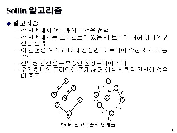
Kruskal 알고리즘(2/3) u 예제 6. 3 0 28 10 1 14 16 5 24 6 2 25 4 18 12 22 3 10 10 1 5 6 2 4 5 0 6 3 (a) (b) (c) 0 0 4 3 (e) 10 1 2 12 14 6 5 4 3 (f) 10 1 16 2 12 5 4 22 6 3 (g) 2 4 12 3 (d) 0 14 6 1 5 2 4 0 10 1 3 14 6 5 0 10 1 16 2 12 0 14 6 5 25 4 22 3 1 16 2 12 (h) Kruskal 알고리즘의 각 단계 35
 0 0 10 1 5 10 2 25 4 25 2 4")
Prim 알고리즘(3/3) 0 0 10 1 5 10 2 25 4 25 2 4 (a) (b) 0 0 1 2 12 3 (d) 25 25 6 2 4 22 3 (c) 1 10 16 5 2 25 6 4 22 1 0 10 5 4 22 6 3 6 10 5 3 10 5 1 5 6 0 12 3 (e) 14 1 16 6 2 4 22 12 3 (f) Prim 알고리즘의 진행 단계 39
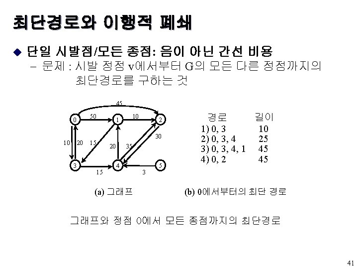
 u Shortest. Path 함수 : 최단 경로의")
하나의 출발점/모든 목표점: 음이 아닌 간선 비용(1/3) u Shortest. Path 함수 : 최단 경로의 길이의 결정 void shortest. Path(int v, int cost[][MAX_VERTICES]), int distance[], int n, short int found[]) {/* distance[i] represents the shortest path from vertex v to I, found[i] is 0 if the shortest path from i has not been found a 1 if it has, cost is the adjacency matrix */ int i, u, w; for (i=0; i<n; i++) { found[i] = FALSE; distance[i] = cost[v][i]; } found[v] = TRUE; distance[v] = 0; for (i=0; i<n-2; i++) { u = choose(distance, n, found); found[u] = TRUE; for (w=0; w<n; w++) if (!found[w]) if (distance[u] + cost[u][w] < distance[w]) distance[w] = distance[u] + cost[u][w]; } } u Shortest. Path의 분석 - n개의 정점을 가진 그래프에 대한 수행시간은 O (n 2) 42
 u 예제 6. 5 Boston Chicago 1200")
하나의 출발점/모든 목표점: 음이 아닌 간선 비용(2/3) u 예제 6. 5 Boston Chicago 1200 San Francisco 800 1 4 1500 3 250 2 1000 Denver 300 5 1000 0 New York 1400 1700 7 Los Angeles 900 New Orleans 1000 6 Miami (a) 방향 그래프 0 0 1 2 3 4 5 6 7 0 300 1000 1 0 800 2 0 1200 3 4 5 0 1500 1000 0 250 0 1700 6 7 900 0 1400 1000 0 (b) 길이-인접 행렬 43
 LA SF 거 리 DEN CHI BOST")
하나의 출발점/모든 목표점: 음이 아닌 간선 비용(3/3) LA SF 거 리 DEN CHI BOST NY MIA ---- [0] [1] [2] [3] 1500 [4] 0 [5] 250 [6] 1 5 1250 0 250 1150 1650 2 6 1250 0 250 1150 1650 3 3 2450 1250 0 250 1150 1650 4 7 3350 2450 1250 0 250 1150 1650 5 2 3350 3250 2450 1250 0 250 1150 1650 6 1 3350 3250 2450 1250 0 250 1150 1650 반복 초기 선택된 정점 NO [7] 방향그래프에 대한 Shortest. Path의 작동 44
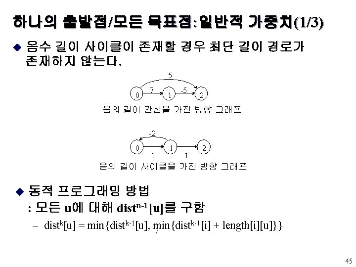
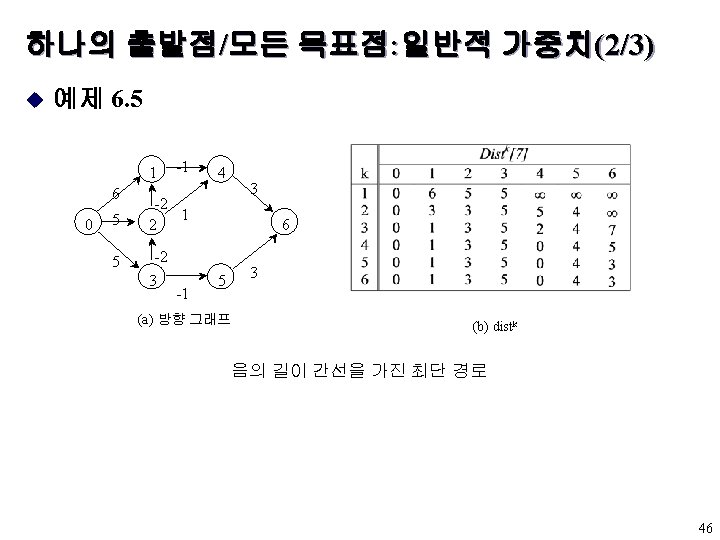
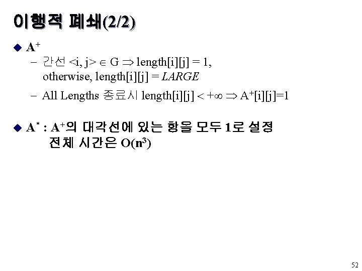
 u Bellman과 Ford 알고리즘 void Bellman. Ford(int n, int")
하나의 출발점/모든 목표점: 일반적 가중치(3/3) u Bellman과 Ford 알고리즘 void Bellman. Ford(int n, int v) { /* single source all destination shortest paths with negative edge lengths. */ for (int I =0; i<n; i++) dist[i] = length[v][i]; /* initialize dist */ for (int k =2; k <= n-1; k++) for (each u such that u != v and u has at least one incoming edge) for (each <i, u> in the edge) if (dist[u] > dist[i] + length[i][u]) dist[u] = dist[i] + length[i][u]; } 최단 경로를 계산하는 Bellman과 Ford 알고리즘 u Bellman. Ford의 분석 - 인접행렬 O(n 3), 인접 리스트 O(ne) 47
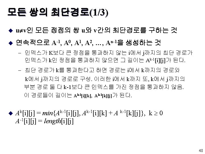
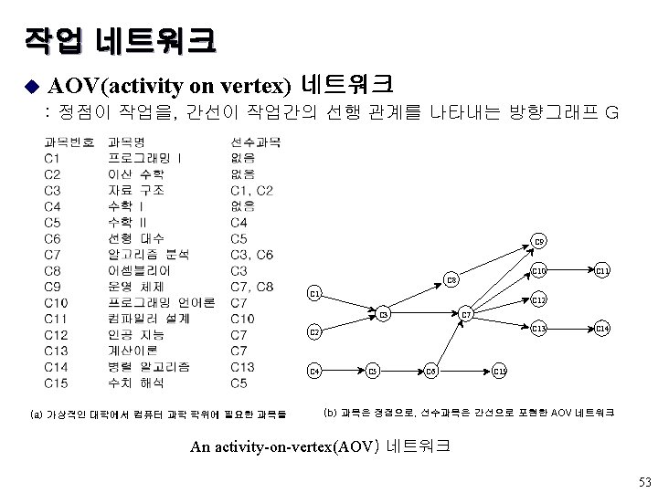
 u u v인 모든 정점의 쌍 u와 v간의 최단경로를 구하는 것")
모든 쌍의 최단경로(2/3) u u v인 모든 정점의 쌍 u와 v간의 최단경로를 구하는 것 Ak[i][j] = min{Ak-1[i][j], Ak-1[i][k] + A k-1[k][j], k 0 A-1[i][j] = length[i][j] void allcosts (int cost[][MAX_VERTICES], int distance[][MAX_VERTICES], int n) { /* 각 정점에서 다른 모든 정점으로의 거리 계산, cost는 인접 행렬, distance는 거리값의 행렬 */} int i, j, k; for (i=0; i<n; i++) for (j=0; j<n; j++) distance[i][j] = cost[i][j]; for (k=0; k<n; k++) for (i=0; i<n; i++) } for (j=0; j<n; j++) if distance[j][k] + distance[k][j] < distance[i][j]) distance[i][j] = distance[i][k] + distance[k][j]; 모든 쌍의 최단경로 u All. Lengths의 분석 - 전체 시간은 O(n 3) 49
 u 예제 6. 6 6 0 1 4 11 A 0")
모든 쌍의 최단경로(3/3) u 예제 6. 6 6 0 1 4 11 A 0 1 2 2 3 -1 2 0 1 0 2 A 0 4 11 6 0 2 3 0 0 1 2 (b) A-1 (a) 방향그래프 0 1 2 0 4 11 6 0 2 3 7 0 (c) A 0 1 2 A 2 0 1 2 0 4 6 0 3 7 6 2 0 0 1 2 0 4 5 0 3 7 6 2 0 A (d) A 1 (e) A 2 모든 쌍의 최단 경로 문제의 예 50

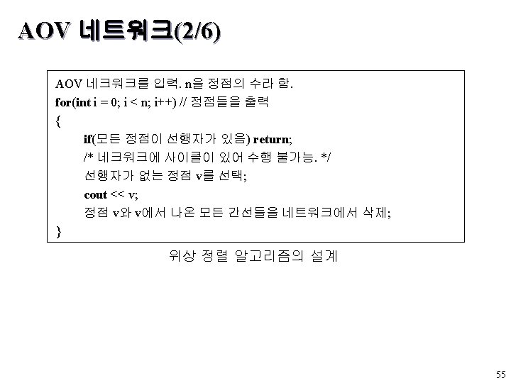
 u Topological. Order의 분석 - 점근적 계산 시간 O (e+n) void top.")
AOV 네트워크(5/6) u Topological. Order의 분석 - 점근적 계산 시간 O (e+n) void top. Sort (hdnodes graph[], int[]) { int i, j, k, top; node. Pointer ptr; /* create a stack of vertices with no predecessors */ top = -1; for (i=0; i<n; i++) if (!graph[i]. count = top); graph[i]. count = top; top = i; } for (i=0; i<n; i++) if (top = = -1) { fprintf(stderr, “n. Network has a cycle. Sort terminated. n”); exit (EXIT_FAILURE); } else { j = top; /* unstack a vertex */ 58
![AOV 네트워크(6/6) top = graph[top]. count; printf (“v%d, ”, j); for (ptr = graph[j].](http://slidetodoc.com/presentation_image/1fe3a5588cb09a980ced0c2e6ca8990b/image-59.jpg "AOV 네트워크(6/6) top = graph[top]. count; printf (“v%d, ”, j); for (ptr = graph[j].")
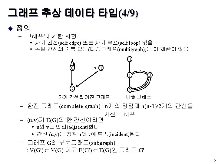
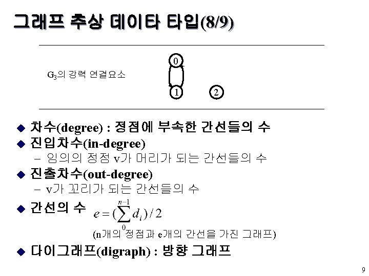
AOV 네트워크(6/6) top = graph[top]. count; printf (“v%d, ”, j); for (ptr = graph[j]. link; ptr = ptr → link) { /* decrease the count of the successor vertices of j*/ } } } k = ptr→vertex; graph[k]. count --; if (!graph[k]. count) { /* add vertex k to the stack */ graph[k]. count = top; top = k; } 위상 정렬 59
![AOE 네트워크(5/8) count first (a) 인접리스트 vertex dur link [0] 0 1 6 [1]](http://slidetodoc.com/presentation_image/1fe3a5588cb09a980ced0c2e6ca8990b/image-64.jpg "AOE 네트워크(5/8) count first (a) 인접리스트 vertex dur link [0] 0 1 6 [1]")
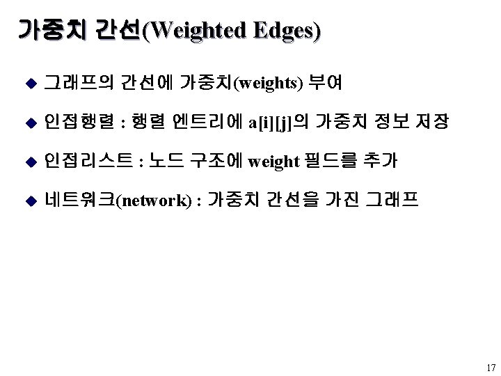
AOE 네트워크(5/8) count first (a) 인접리스트 vertex dur link [0] 0 1 6 [1] 1 4 1 0 [2] 1 4 1 0 [3] 1 5 2 0 [4] 2 6 9 [5] 1 7 4 0 [6] 1 8 2 0 [7] 2 8 4 0 [8] 2 2 4 7 7 3 5 0 0 0 (b) ee의 계산 64
![AOE 네트워크(6/8) u 가장 늦은 시간의 계산 - le[j] = min { le[i] -](http://slidetodoc.com/presentation_image/1fe3a5588cb09a980ced0c2e6ca8990b/image-65.jpg "AOE 네트워크(6/8) u 가장 늦은 시간의 계산 - le[j] = min { le[i] -")
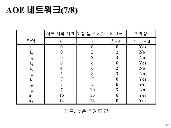
AOE 네트워크(6/8) u 가장 늦은 시간의 계산 - le[j] = min { le[i] - <j, i>의 기간 } i P(j) (S(j)는 j의 직속 후속자들의 집합) le[8]=ee[8]=18 le[6]=min{le[8]-2}=16 le[7]=min{le[8]-4}=14 le[4]=min{le[6]-9, le[7]-7}=7 le[1]=min{le[4]-1}=6 le[2]=min{le[4]-1}=6 le[5]=min{le[7]-4}=10 le[3]=min{le[5]-2}=8 le[0]=min{le[1]-6, le[2]-4, le[3]-5}=0 AOE 네트워크에 대한 le의 계산 65
- Slides: 67