9 0 Speech Recognition Updates MinimumClassificationError MCE and

9. 0 Speech Recognition Updates

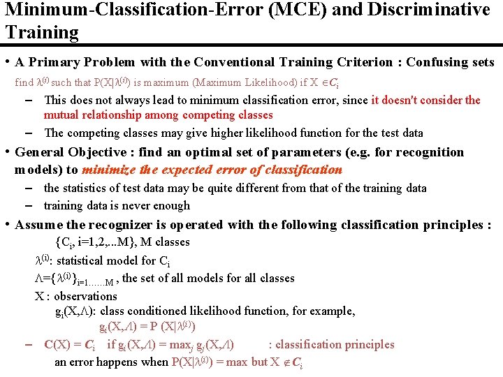
Minimum-Classification-Error (MCE) and Discriminative Training • A Primary Problem with the Conventional Training Criterion : Confusing sets find (i) such that P(X| (i)) is maximum (Maximum Likelihood) if X Ci – This does not always lead to minimum classification error, since it doesn't consider the mutual relationship among competing classes – The competing classes may give higher likelihood function for the test data • General Objective : find an optimal set of parameters (e. g. for recognition models) to minimize the expected error of classification – the statistics of test data may be quite different from that of the training data – training data is never enough • Assume the recognizer is operated with the following classification principles : {Ci, i=1, 2, . . . M}, M classes (i): statistical model for Ci ={ (i)}i=1……M , the set of all models for all classes X : observations gi(X, ): class conditioned likelihood function, for example, gi(X, ) = P (X| (i)) – C(X) = Ci if gi(X, ) = maxj gj(X, ) : classification principles an error happens when P(X| (i)) = max but X Ci

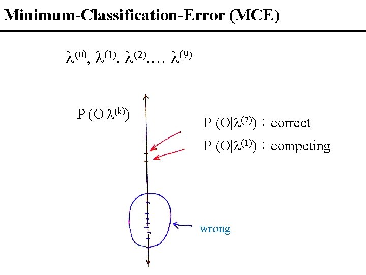
Minimum-Classification-Error (MCE) (0), (1), (2), … (9) P (O| (k)) P (O| (7))：correct P (O| (1))：competing wrong

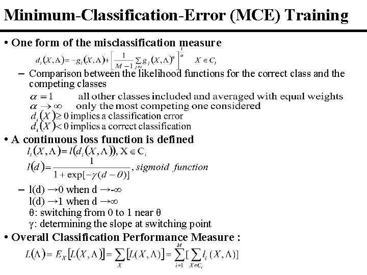
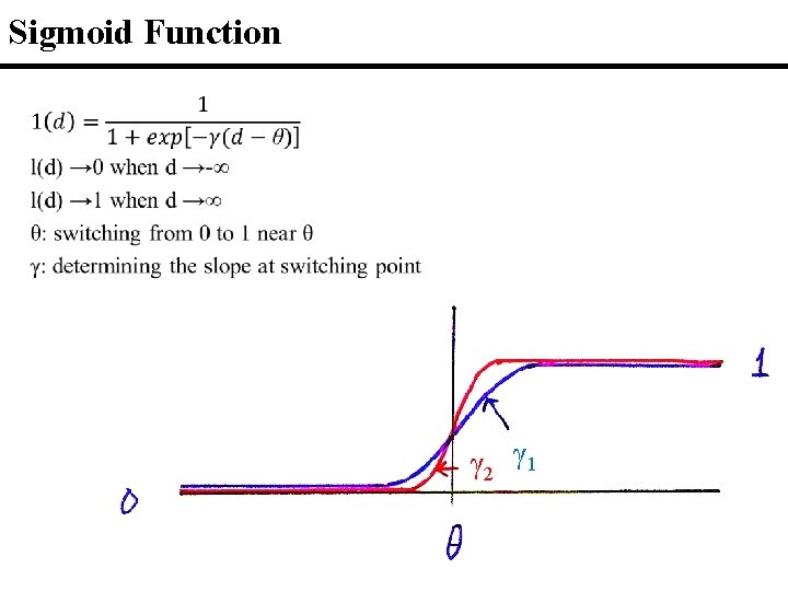
Minimum-Classification-Error (MCE) Training • One form of the misclassification measure – Comparison between the likelihood functions for the correct class and the competing classes • A continuous loss function is defined – l(d) → 0 when d →-∞ l(d) → 1 when d →∞ θ: switching from 0 to 1 near θ γ: determining the slope at switching point • Overall Classification Performance Measure :

Sigmoid Function 0 γ 2 γ 1

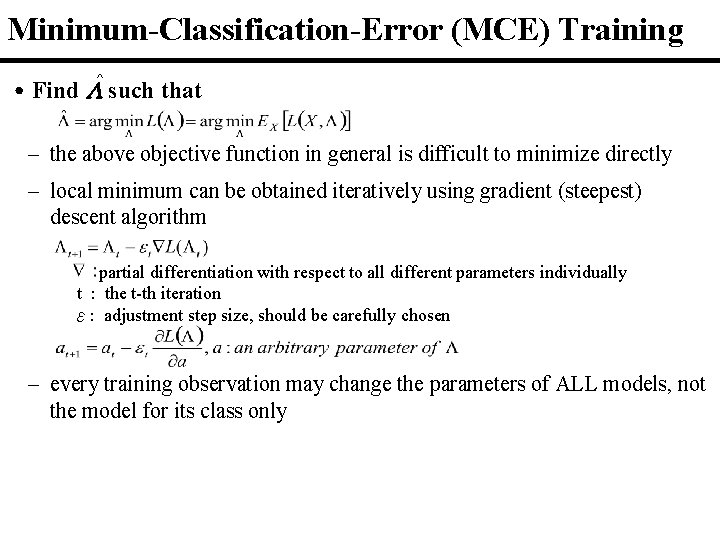
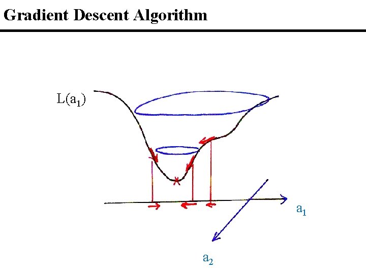
Minimum-Classification-Error (MCE) Training ^ ˙Find such that – the above objective function in general is difficult to minimize directly – local minimum can be obtained iteratively using gradient (steepest) descent algorithm partial differentiation with respect to all different parameters individually t : the t-th iteration ε: adjustment step size, should be carefully chosen – every training observation may change the parameters of ALL models, not the model for its class only

Gradient Descent Algorithm L(a 1) a 1 a 2

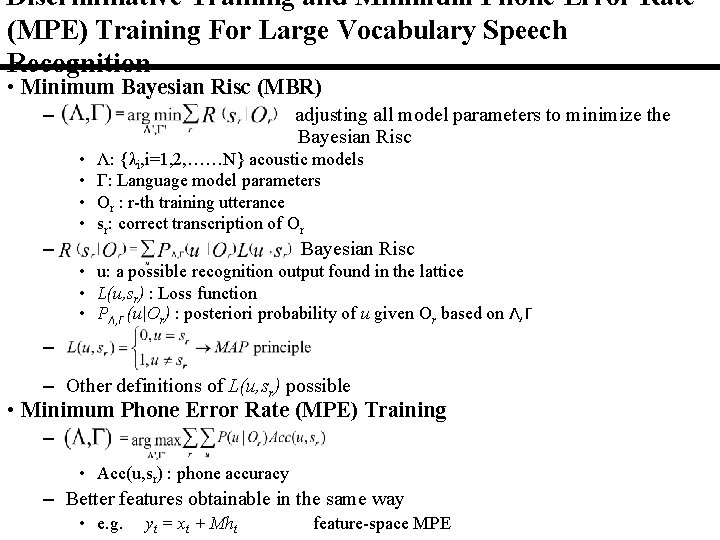
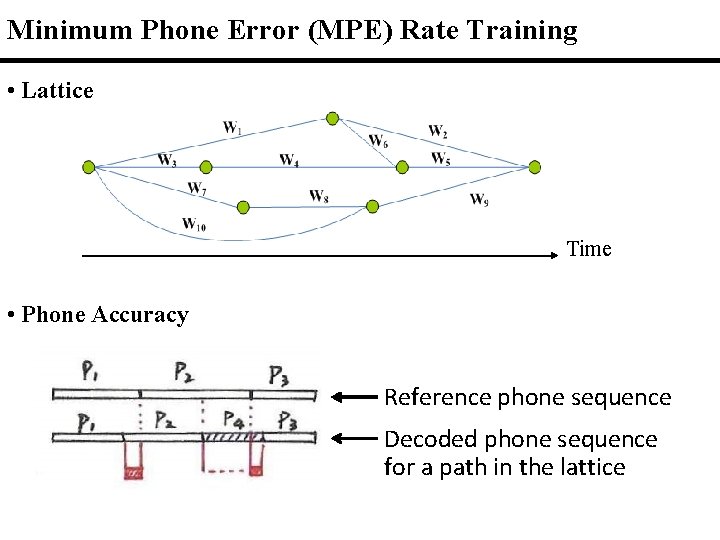
Discriminative Training and Minimum Phone Error Rate (MPE) Training For Large Vocabulary Speech Recognition • Minimum Bayesian Risc (MBR) – • • adjusting all model parameters to minimize the Bayesian Risc Λ: {λi, i=1, 2, ……N} acoustic models Γ: Language model parameters Or : r-th training utterance sr: correct transcription of Or – Bayesian Risc • u: a possible recognition output found in the lattice • L(u, sr) : Loss function • PΛ, Γ (u|Or) : posteriori probability of u given Or based on Λ, Γ – – Other definitions of L(u, sr) possible • Minimum Phone Error Rate (MPE) Training – • Acc(u, sr) : phone accuracy – Better features obtainable in the same way • e. g. yt = xt + Mht feature-space MPE

Minimum Phone Error (MPE) Rate Training • Lattice Time • Phone Accuracy Reference phone sequence Decoded phone sequence for a path in the lattice

References for MCE, MPE and Discriminative Training • “ Minimum Classification Error Rate Methods for Speech Recognition”, IEEE Trans. Speech and Audio Processing, May 1997 • “Segmental Minimum Bayes-Rick Decoding for Automatic Speech Recognition”, IEEE Trans. Speech and Audio Processing, 2004 • “Minimum Phone Error and I-smoothing for Improved Discriminative Training”, International Conference on Acoustics, Speech and Signal Processing, 2002 • “Discriminative Training for Automatic Speech Recognition”, IEEE Signal Processing Magazine, Nov 2012

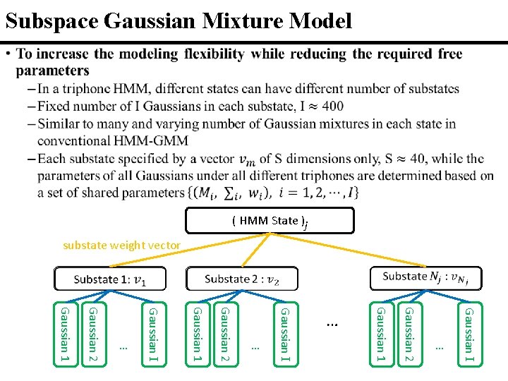
Subspace Gaussian Mixture Model • ( HMM State )j substate weight vector Gaussian I Gaussian 1 Gaussian 2 … Gaussian I …

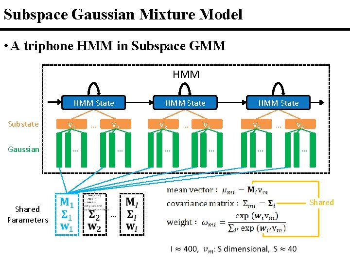
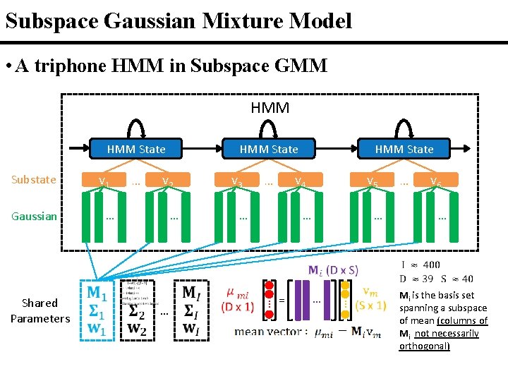
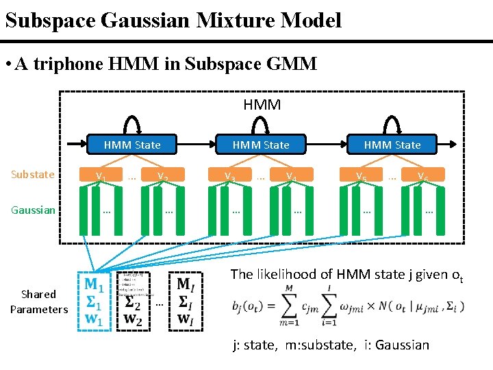
Subspace Gaussian Mixture Model • A triphone HMM in Subspace GMM HMM State Substate Gaussian Shared Parameters v 1 … HMM State v 2 … … v 3 … … HMM State v 4 … v 5 … … v 6 … Shared …

Subspace Gaussian Mixture Model • A triphone HMM in Subspace GMM HMM State Substate Gaussian … v 2 … … HMM State v 4 … … v 5 … = … … v 3 … Shared Parameters v 1 HMM State … v 6 … Mi is the basis set spanning a subspace of mean (columns of Mi not necessarily orthogonal)

Subspace Gaussian Mixture Model • A triphone HMM in Subspace GMM HMM State Substate Gaussian v 1 … HMM State v 2 … … v 3 … … HMM State v 4 … v 5 … … v 6 … The likelihood of HMM state j given ot Shared Parameters … j: state, m: substate, i: Gaussian

References for Subspace Gaussian Mixture Model • "The Subspace Gaussian Mixture Model– a Structured Model for Speech Recognition", D. Povey, Lukas Burget et. al Computer Speech and Language, 2011 • "A Symmetrization of the Subspace Gaussian Mixture Model", Daniel Povey, Martin Karafiat, Arnab Ghoshal, Petr Schwarz, ICASSP 2011 • "Subspace Gaussian Mixture Models for Speech Recognition", D. Povey, Lukas Burget et al. , ICASSP 2010 • "A Tutorial-Style Introduction To Subspace Gaussian Mixture Models For Speech Recognition", Microsoft Research technical report MSR-TR-2009 -111

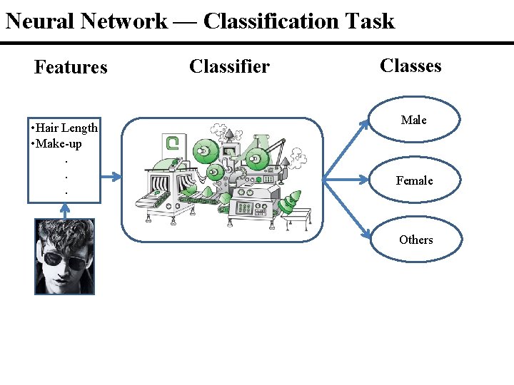
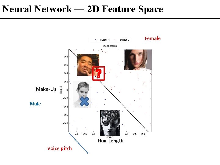
Neural Network — Classification Task Features • Hair Length • Make-up. . . Classifier Classes Male Classifier Female Others

Neural Network — 2 D Feature Space Female Make-Up Male Hair Length Voice pitch

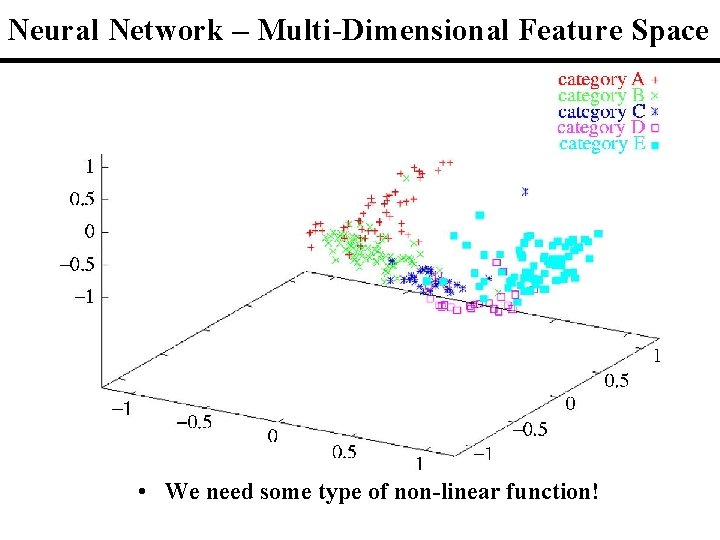
Neural Network ‒ Multi-Dimensional Feature Space • We need some type of non-linear function!

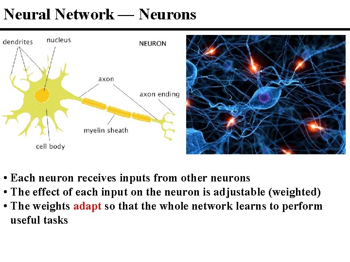
Neural Network — Neurons • Each neuron receives inputs from other neurons • The effect of each input on the neuron is adjustable (weighted) • The weights adapt so that the whole network learns to perform useful tasks

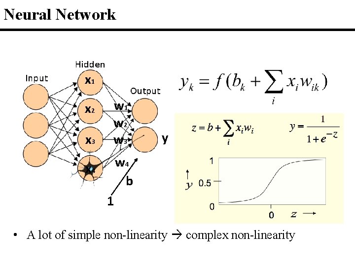
Neural Network x 1 x 2 x 3 w 1 w 2 w 3 y w 4 b x 4 1 • A lot of simple non-linearity complex non-linearity

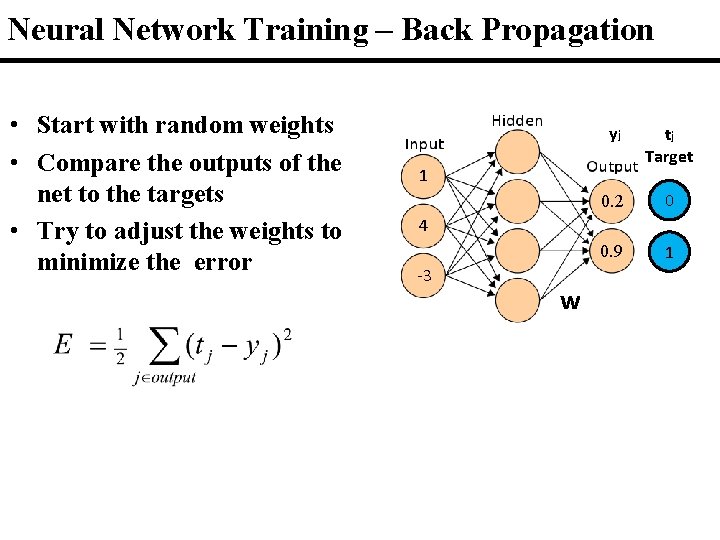
Neural Network Training – Back Propagation • Start with random weights • Compare the outputs of the net to the targets • Try to adjust the weights to minimize the error yj tj Target 0. 2 0 0. 9 1 1 4 -3 w

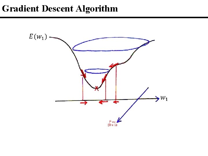
Gradient Descent Algorithm

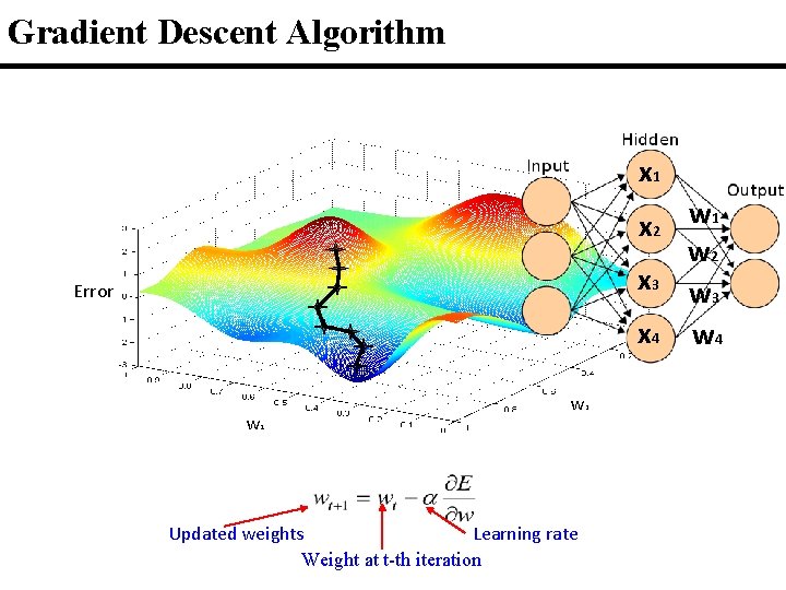
Gradient Descent Algorithm x 1 x 2 w 1 w 2 x 3 w 3 x 4 w 4 Error w w 1 Updated weights Learning rate Weight at t-th iteration 2

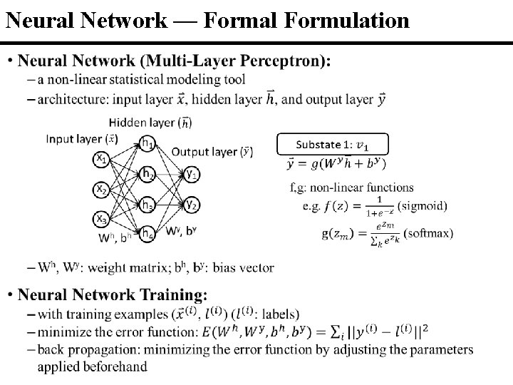
Neural Network — Formal Formulation • •

References for Neural Network • Rumelhart, David E. ; Hinton, Geoffrey E. , Williams, Ronald J. "Learning representations by back-propagating errors". Nature, 1986. • Alpaydın, Ethem. Introduction to machine learning (2 nd ed. ), MIT Press, 2010. • Albert Nigrin, Neural Networks for Pattern Recognition(1 st ed. ). A Bradford Book, 1993. • Reference: Neural Networks for Machine Learning course by Geoffrey Hinton, Coursera

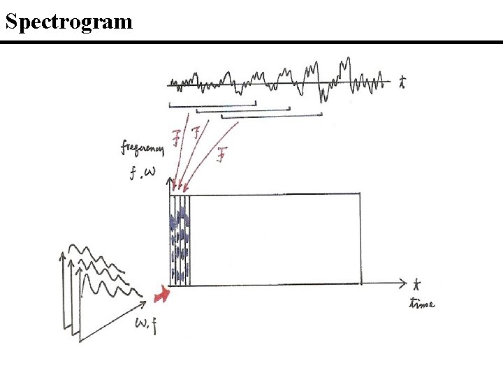
Spectrogram

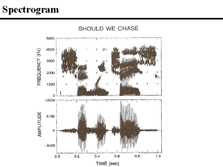
Spectrogram

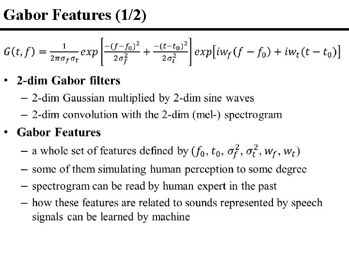
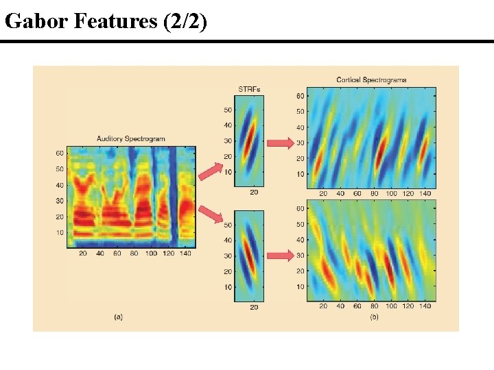
Gabor Features (1/2) •

Gabor Features (2/2)

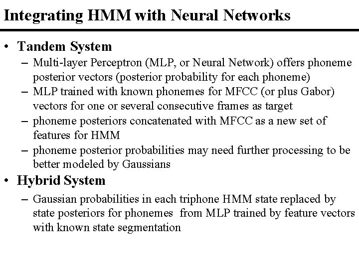
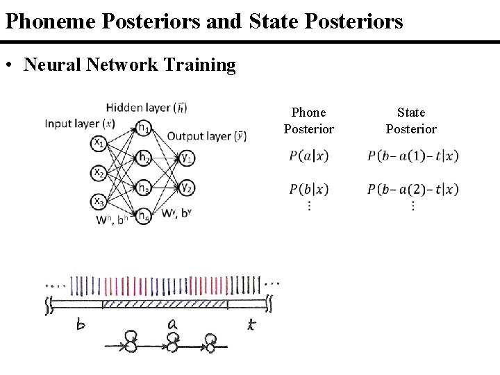
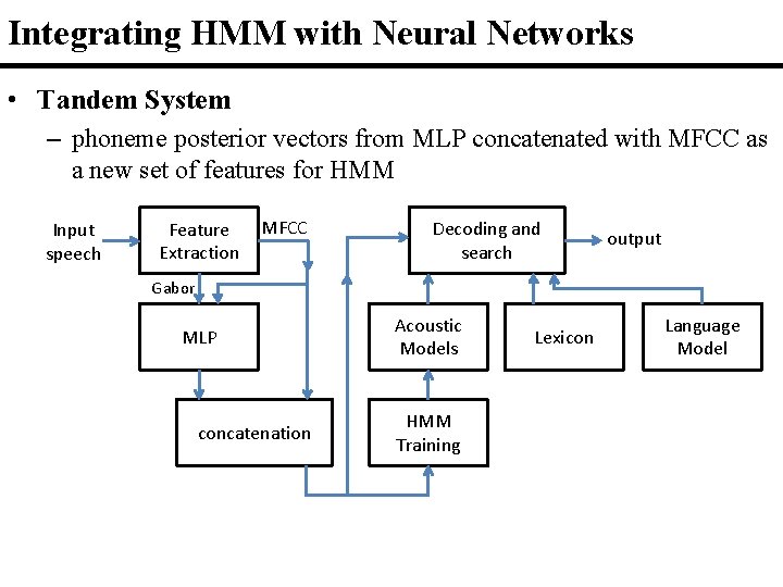
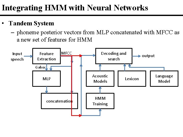
Integrating HMM with Neural Networks • Tandem System – Multi-layer Perceptron (MLP, or Neural Network) offers phoneme posterior vectors (posterior probability for each phoneme) – MLP trained with known phonemes for MFCC (or plus Gabor) vectors for one or several consecutive frames as target – phoneme posteriors concatenated with MFCC as a new set of features for HMM – phoneme posterior probabilities may need further processing to be better modeled by Gaussians • Hybrid System – Gaussian probabilities in each triphone HMM state replaced by state posteriors for phonemes from MLP trained by feature vectors with known state segmentation

Phoneme Posteriors and State Posteriors • Neural Network Training • Phone Posterior State Posterior

Integrating HMM with Neural Networks • Tandem System – phoneme posterior vectors from MLP concatenated with MFCC as a new set of features for HMM Input speech Feature Extraction MFCC Decoding and search output Gabor MLP concatenation Acoustic Models HMM Training Lexicon Language Model

Integrating HMM with Neural Networks • Tandem System – phoneme posterior vectors from MLP concatenated with MFCC as a new set of features for HMM Input speech Feature Extraction MFCC Decoding and search output Gabor MLP concatenation Acoustic Models HMM Training Lexicon Language Model

References • References for Gabor Features and Tandem System – Richard M. Stern & Nelson Morgan, “Hearing Is Believing”, IEEE SIGNAL PROCESSING MAGAZINE, NOVEMBER 2012 – Hermansky, H. , Ellis, D. P. W. , Sharma, S. , “Tandem Connectionist Feature Extraction For Conventional Hmm Systems”, in Proc. ICASSP 2000. – Ellis, D. P. W. and Singh, R. and Sivadas, S. , “Tandem acoustic modeling in large-vocabulary recognition”, in Proc. ICASSP 2001. – “Improved Tonal Language Speech Recognition by Integrating Spectro-Temporal Evidence and Pitch Information with Properly Chosen Tonal Acoustic Units”, Interspeech, Florence, Italy, Aug 2011, pp. 2293 -2296.

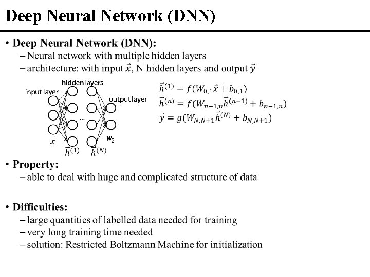
Deep Neural Network (DNN) •

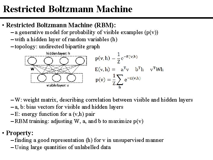
Restricted Boltzmann Machine • Restricted Boltzmann Machine (RBM): – a generative model for probability of visible examples (p(v)) – with a hidden layer of random variables (h) – topology: undirected bipartite graph – W: weight matrix, describing correlation between visible and hidden layers – a, b: bias vectors for visible and hidden layers – E: energy function for a (v, h) pair – RBM training: adjusting W, a, and b to maximize p(v) • Property: – finding a good representation (h) for v in unsupervised manner – Using large quantities of unlabelled data

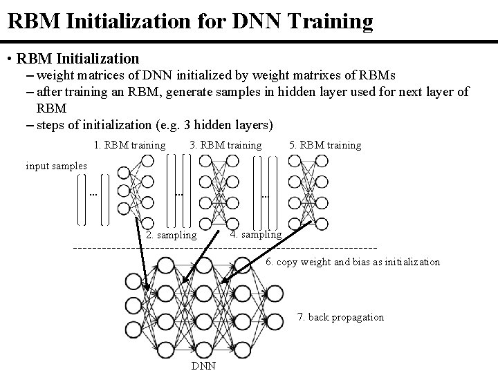
RBM Initialization for DNN Training • RBM Initialization – weight matrices of DNN initialized by weight matrixes of RBMs – after training an RBM, generate samples in hidden layer used for next layer of RBM – steps of initialization (e. g. 3 hidden layers) 1. RBM training 3. RBM training 5. RBM training input samples … … … 2. sampling 4. sampling 6. copy weight and bias as initialization 7. back propagation DNN

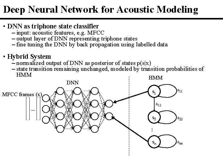
Deep Neural Network for Acoustic Modeling • DNN as triphone state classifier – input: acoustic features, e. g. MFCC – output layer of DNN representing triphone states – fine tuning the DNN by back propagation using labelled data • Hybrid System – normalized output of DNN as posterior of states p(s|x) – state transition remaining unchanged, modeled by transition probabilities of HMM DNN MFCC frames (x) … s 1 a 12 s 2 a 22 … sn ann

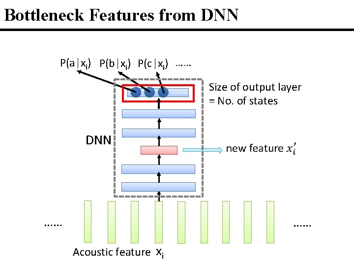
Bottleneck Features from DNN P(a|xi) P(b|xi) P(c|xi) …… …… Size of output layer = No. of states DNN …… …… Acoustic feature xi

References for DNN • Context-Dependent Pre-trained Deep Neural Networks for Large Vocabulary Speech Recognition – George E. Dahl, Dong Yu, Deng Li, and Alex Acero – IEEE Trans. on Audio, Speech and Language Processing, Jan, 2012 • A fast learning algorithm for deep belief – Hinton, G. E. , Osindero, S. and Teh, Y – Neural Computation, 18, pp 1527 -1554, 2006 • Deep Neural Networks for Acoustic Modeling in Speech Recognition – G. Hinton, L. Deng, D. Yu, G. Dahl, A. Mohamed, N. Jaitly, A. Senior, V. Vanhoucke, P. Nguyen, T. Sainath, and B. Kingsbury – IEEE Signal Processing Magazine, 29, November 2012 • Deep Learning and Its Applications to Signal and Information Processing – IEEE Signal Processing Magazine, Jan 2011 • Improved Bottleneck Features Using Pretrained Deep Neural Networks – Yu, Dong, and Michael L. Seltzer – Interspeech 2011 • Extracting deep bottleneck features using stacked auto-encoders – Gehring, Jonas, et al. – ICASSP 2013

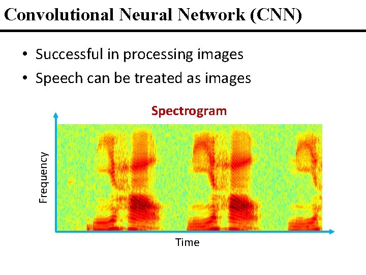
Convolutional Neural Network (CNN) • Successful in processing images • Speech can be treated as images Frequency Spectrogram Time

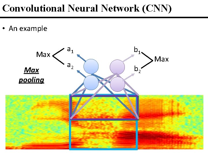
Convolutional Neural Network (CNN) • An example Max pooling a 1 a 2 b 1 b 2 Max

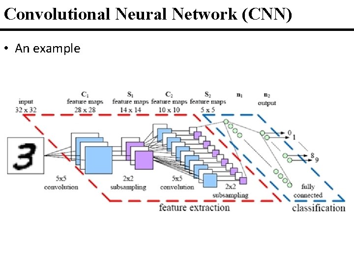
Convolutional Neural Network (CNN) • An example CNN

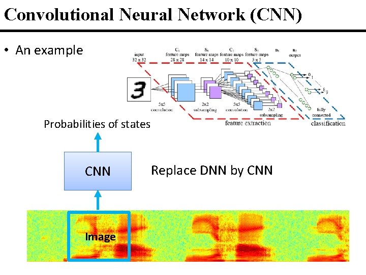
Convolutional Neural Network (CNN) CNN • An example Probabilities of states CNN Image Replace DNN by CNN

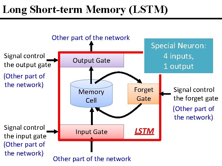
Long Short-term Memory (LSTM) Other part of the network Signal control the output gate (Other part of the network) Signal control the input gate (Other part of the network) Output Gate Special Neuron: 4 inputs, 1 output Memory Cell Forget Gate Input Gate LSTM Other part of the network Signal control the forget gate (Other part of the network)

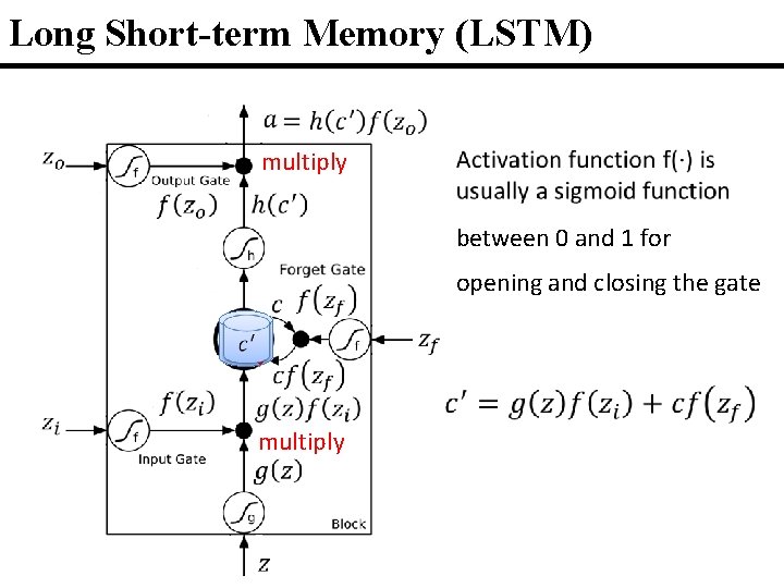
Long Short-term Memory (LSTM) multiply between 0 and 1 for opening and closing the gate c multiply

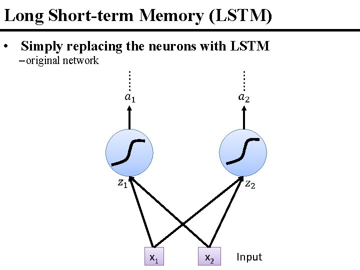
Long Short-term Memory (LSTM) • Simply replacing the neurons with LSTM – original network …… …… x 1 x 2 Input

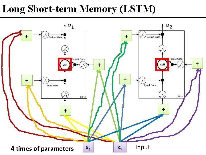
Long Short-term Memory (LSTM) + + + + 4 times of parameters x 1 x 2 Input

References Convolutional Neural Network (CNN) • Convolutional Neural Network for Image processing – Zeiler, M. D. , & Fergus, R. (2014). “Visualizing and understanding convolutional networks. ” In Computer Vision–ECCV 2014 • Convolutional Neural Network for speech processing – Tóth, László. "Convolutional deep maxout networks for phone recognition. " Proc. Interspeech. 2014. • Convolutional Neural Network for text processing – Shen, Yelong, et al. "A latent semantic model with convolutional-pooling structure for information retrieval. " Proceedings of the 23 rd ACM International Conference on Information and Knowledge Management. ACM, 2014. Long Short-term Memory (LSTM) • Graves, N. Jaitly, A. Mohamed. “Hybrid Speech Recognition with Deep Bidirectional LSTM”, ASRU 2013. • Graves, Alex, and Navdeep Jaitly. "Towards end-to-end speech recognition with recurrent neural networks. " Proceedings of the 31 st International Conference on Machine Learning (ICML-14). 2014.

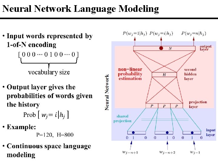
Neural Network Language Modeling • vocabulary size

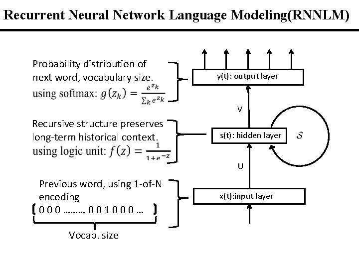
Recurrent Neural Network Language Modeling(RNNLM) Probability distribution of next word, vocabulary size. y(t): output layer V Recursive structure preserves long-term historical context. s(t): hidden layer U Previous word, using 1 -of-N encoding 0 0 0 ……… 0 0 1 0 0 0 … Vocab. size x(t): input layer

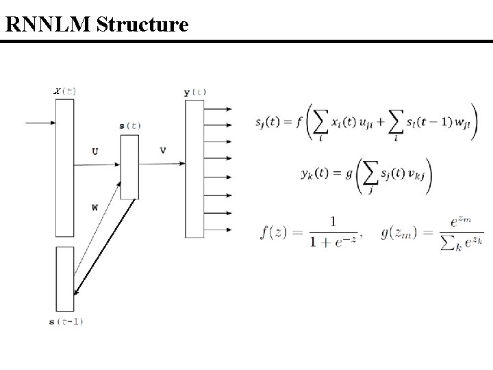
RNNLM Structure x

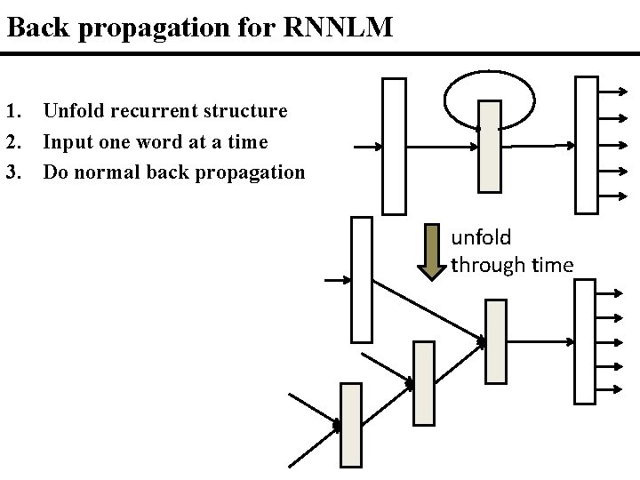
Back propagation for RNNLM 1. Unfold recurrent structure 2. Input one word at a time 3. Do normal back propagation unfold through time

References for RNNLM • Yoshua Bengio, Rejean Ducharme and Pascal Vincent. “A neural probabilistic language model, ” Journal of Machine Learning Research, 3: 1137– 1155, 2003 • Holger Schwenk. “Continuous space language models, ” Computer Speech and Language, vol. 21, pp. 492– 518, 2007 • Tomáš Mikolov, Martin Karafiát, Lukáš Burget, Jan Černocký and Sanjeev Khudanpur. “Recurrent neural network based language model, ” in Interspeech 2010 • Mikolov Tomáš et al, “Extensions of Recurrent Neural Network Language Model”, ICASSP 2011. • Mikolov Tomáš et al, “Context Dependent Recurrent Neural Network Language Model”, IEEE SLT 2012.

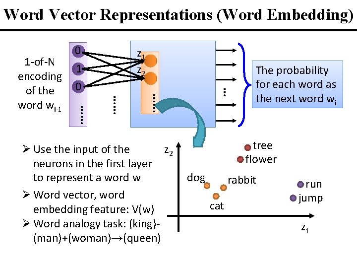
Word Vector Representations (Word Embedding) 0 … …… …… …… 1 -of-N 1 encoding 0 of the word wi-1 z 1 z 2 Ø Use the input of the z 2 neurons in the first layer to represent a word w Ø Word vector, word embedding feature: V(w) Ø Word analogy task: (king)(man)+(woman)→(queen) The probability for each word as the next word wi tree flower dog rabbit cat run jump z 1

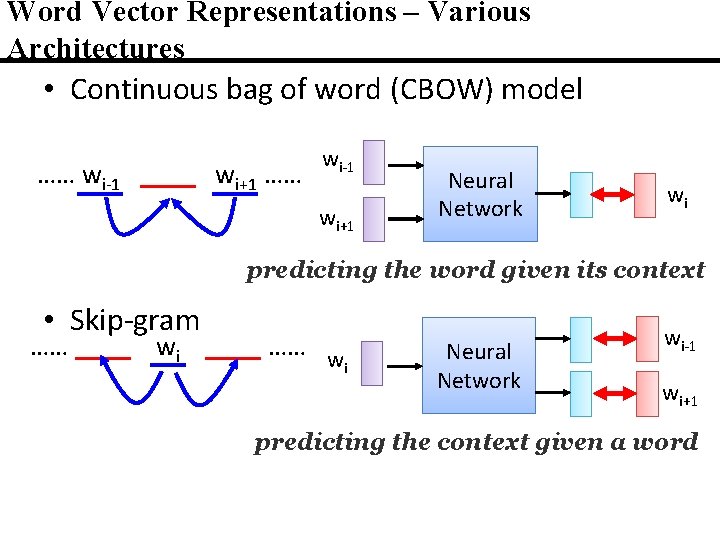
Word Vector Representations – Various Architectures • Continuous bag of word (CBOW) model …… wi-1 ____ wi+1 …… wi-1 wi+1 Neural Network wi predicting the word given its context • Skip-gram …… ____ wi ____ …… w i Neural Network wi-1 wi+1 predicting the context given a word

References for Word Vector Representations • Tomas Mikolov, Kai Chen, Greg Corrado, and Jeffrey Dean. ”Efficient Estimation of Word Representations in Vector Space. ” In Proceedings of Workshop at ICLR, 2013. • Tomas Mikolov, Ilya Sutskever, Kai Chen, Greg Corrado, and Jeffrey Dean. ”Distributed Representations of Words and Phrases and their Compositionality. ” In Proceedings of NIPS, 2013. • Tomas Mikolov, Wen-tau Yih, and Geoffrey Zweig. ”Linguistic Regularities in Continuous Space Word Representations. ” In Proceedings of NAACL HLT, 2013.

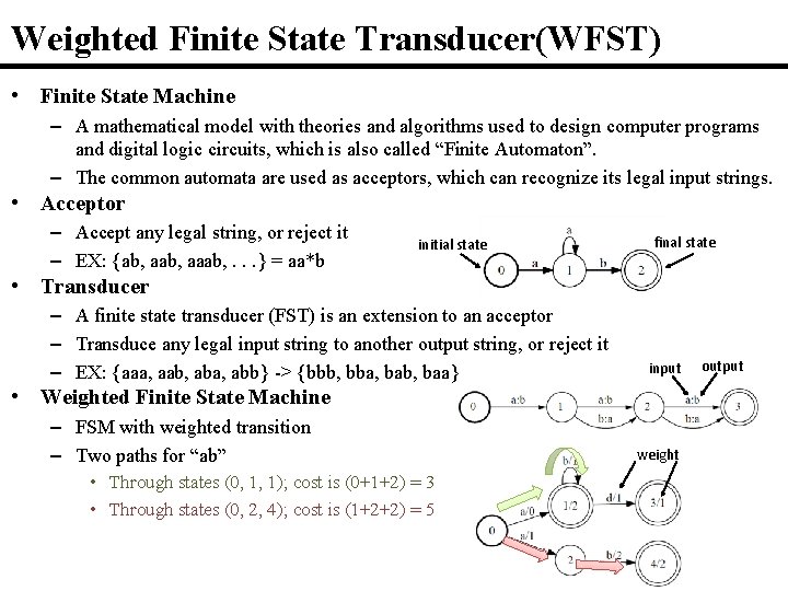
Weighted Finite State Transducer(WFST) • Finite State Machine – A mathematical model with theories and algorithms used to design computer programs and digital logic circuits, which is also called “Finite Automaton”. – The common automata are used as acceptors, which can recognize its legal input strings. • Acceptor – Accept any legal string, or reject it – EX: {ab, aaab, . . . } = aa*b initial state final state • Transducer – A finite state transducer (FST) is an extension to an acceptor – Transduce any legal input string to another output string, or reject it – EX: {aaa, aab, aba, abb} -> {bbb, bba, bab, baa} input • Weighted Finite State Machine – FSM with weighted transition – Two paths for “ab” • Through states (0, 1, 1); cost is (0+1+2) = 3 • Through states (0, 2, 4); cost is (1+2+2) = 5 weight output

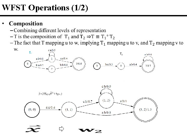
WFST Operations (1/2) •

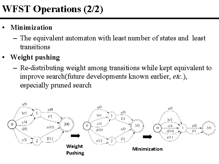
WFST Operations (2/2) • Minimization – The equivalent automaton with least number of states and least transitions • Weight pushing – Re-distributing weight among transitions while kept equivalent to improve search(future developments known earlier, etc. ), especially pruned search Weight Pushing Minimization

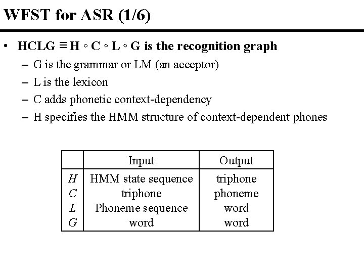
WFST for ASR (1/6) • HCLG ≡ H ◦ C ◦ L ◦ G is the recognition graph – – G is the grammar or LM (an acceptor) L is the lexicon C adds phonetic context-dependency H specifies the HMM structure of context-dependent phones H C L G Input HMM state sequence triphone Phoneme sequence word Output triphoneme word

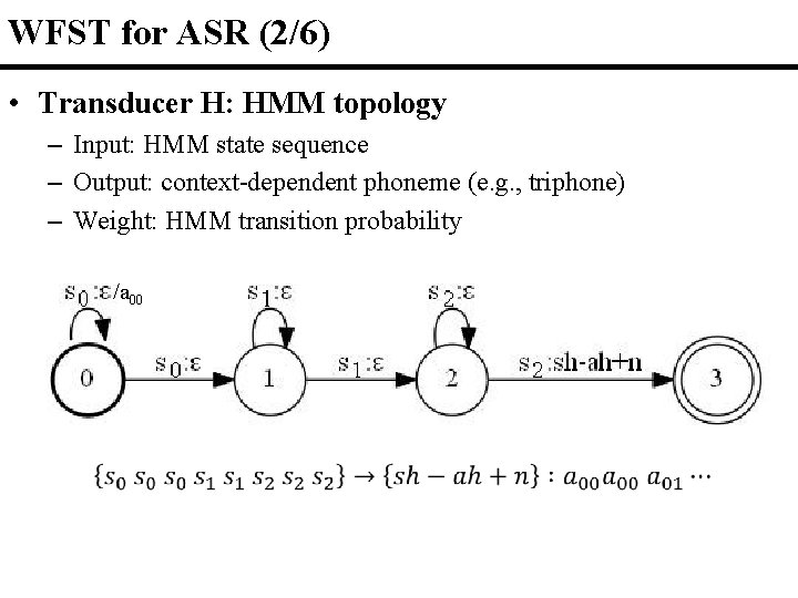
WFST for ASR (2/6) • Transducer H: HMM topology – Input: HMM state sequence – Output: context-dependent phoneme (e. g. , triphone) – Weight: HMM transition probability /a 00

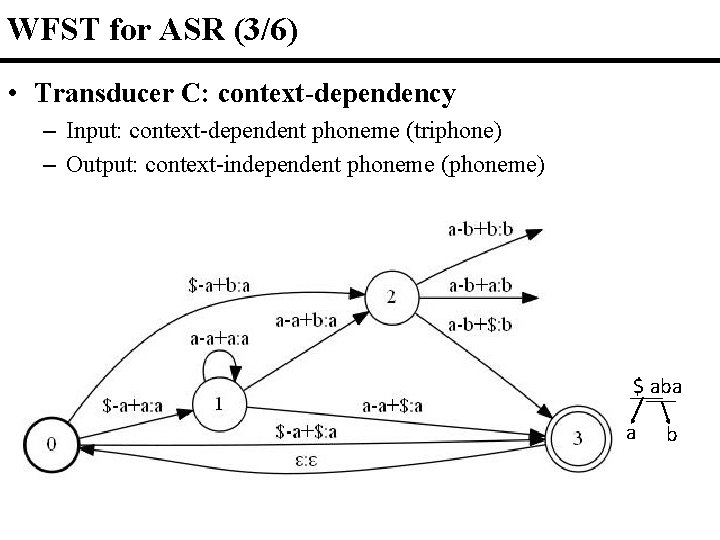
WFST for ASR (3/6) • Transducer C: context-dependency – Input: context-dependent phoneme (triphone) – Output: context-independent phoneme (phoneme) $ aba a b

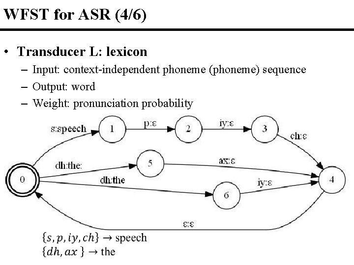
WFST for ASR (4/6) • Transducer L: lexicon – Input: context-independent phoneme (phoneme) sequence – Output: word – Weight: pronunciation probability

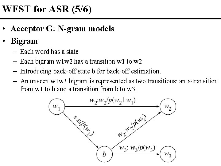
WFST for ASR (5/6) • Acceptor G: N-gram models • Bigram – – Each word has a state Each bigram w 1 w 2 has a transition w 1 to w 2 Introducing back-off state b for back-off estimation. An unseen w 1 w 3 bigram is represented as two transitions: an ε-transition from w 1 to b and a transition from b to w 3.

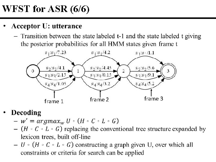
WFST for ASR (6/6) • frame 1 frame 2 frame 3

References • WFST – Mehryar Mohri, “Finite-state transducers in language and speech processing, ”Comput. Linguist. , vol. 23, no. 2, pp. 269– 311, 1997. • WFST for LVCSR – Mehryar Mohri, Fernando Pereira, and Michael Riley, “Weighted automata in text and speech processing, ” in European Conference on Artificial Intelligence. 1996, pp. 46– 50, John Wiley and Sons. – Mehryar Mohri, Fernando C. Pereira, and Michael Riley, “Speech Recognition with Weighted Finite-State Transducers, ” in Springer Handbook of Speech Processing, Jacob Benesty, Mohan M. Sondhi, and Yiteng A. Huang, Eds. , pp. 559– 584. Springer Berlin Heidelberg, Secaucus, NJ, USA, 2008.

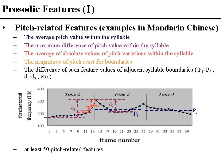
Prosodic Features (І) • Pitch-related Features (examples in Mandarin Chinese) – – – The average pitch value within the syllable The maximum difference of pitch value within the syllable The average of absolute values of pitch variations within the syllable The magnitude of pitch reset for boundaries The difference of such feature values of adjacent syllable boundaries ( P 1 -P 2 , d 1 -d 2 , etc. ) d 1 – at least 50 pitch-related features d 2 P 1 P 2

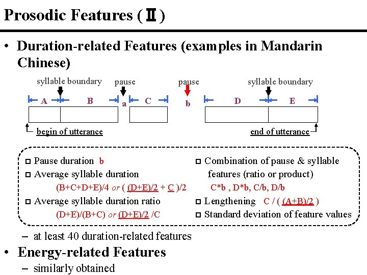
Prosodic Features (Ⅱ) • Duration-related Features (examples in Mandarin Chinese) syllable boundary A pause B a pause C b begin of utterance p Pause duration b syllable boundary D E end of utterance p Combination of pause & syllable features (ratio or product) (B+C+D+E)/4 or ( (D+E)/2 + C )/2 C*b , D*b, C/b, D/b p Lengthening C / ( (A+B)/2 ) p Average syllable duration ratio p Standard deviation of feature values (D+E)/(B+C) or (D+E)/2 /C p Average syllable duration – at least 40 duration-related features • Energy-related Features – similarly obtained

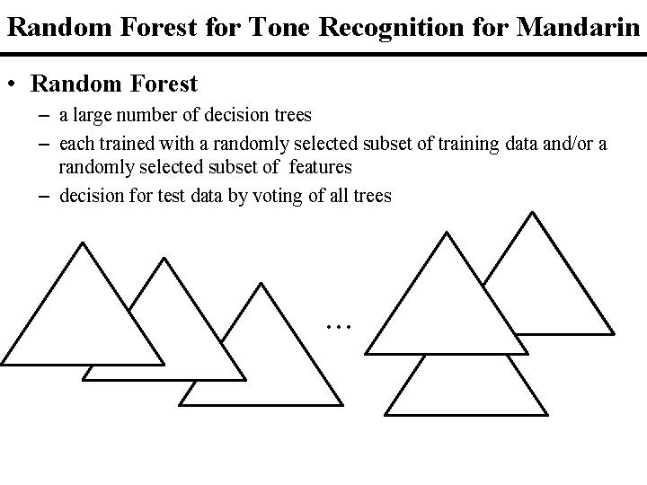
Random Forest for Tone Recognition for Mandarin • Random Forest – a large number of decision trees – each trained with a randomly selected subset of training data and/or a randomly selected subset of features – decision for test data by voting of all trees • • •

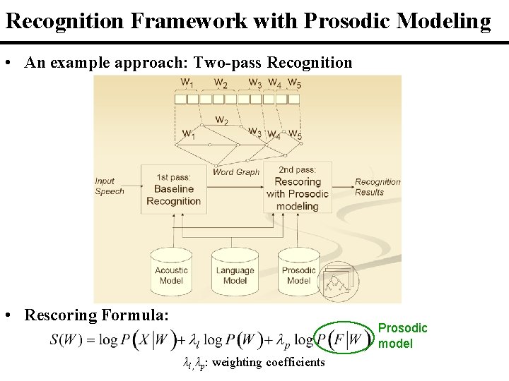
Recognition Framework with Prosodic Modeling • An example approach: Two-pass Recognition • Rescoring Formula: Prosodic model λl , λp: weighting coefficients

References • Prosody – “Improved Large Vocabulary Mandarin Speech Recognition by Selectively Using Tone Information with a Two-stage Prosodic Model”, Interspeech, Brisbane, Australia, Sep 2008, pp. 1137 -1140 – “Latent Prosodic Modeling (LPM) for Speech with Applications in Recognizing Spontaneous Mandarin Speech with Disfluencies”, International Conference on Spoken Language Processing, Pittsburgh, U. S. A. , Sep 2006. – “Improved Features and Models for Detecting Edit Disfluencies in Transcribing Spontaneous Mandarin Speech”, IEEE Transactions on Audio, Speech and Language Processing, Vol. 17, No. 7, Sep 2009, pp. 1263 -1278. • Random Forest – http: //stat-www. berkeley. edu/users/breiman/Random. Forests/cc_home. htm – http: //stat-www. berkeley. edu/users/breiman/Random. Forests/cc_papers. htm

Personalized Recognizer and Social Networks • Personalized recognizer is feasible today – Smart phone user is personal • each smart phone used by a single user • user identification is known once the smart phone is turned on – Personal corpus is available • Audio data easily collected at server • Text data available on social networks

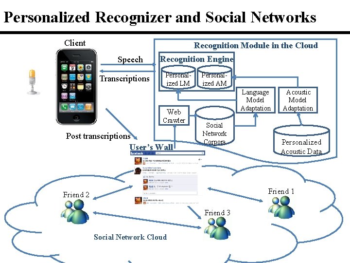
Personalized Recognizer and Social Networks Client Recognition Module in the Cloud Speech Transcriptions Recognition Engine Personal- Personalized LM ized AM Language Model Adaptation Web Crawler Post transcriptions User’s Wall Social Network Corpora Acoustic Model Adaptation Personalized Acoustic Data Friend 1 Friend 2 Friend 3 Social Network Cloud

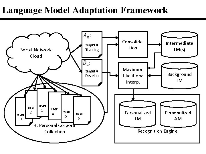
Language Model Adaptation Framework target u Training Social Network Cloud target u Develop user 1 2 4 user 3 user 5 H: Personal Corpora Collection user 6 Consolidation Intermediate LM(s) Maximum Likelihood Interp. Background LM Personalized AM Recognition Engine

References for Personalized Recognizer • “Recurrent Neural Network Based Language Model Personalization by Social Network Crowdsourcing”, Interspeech 2013. • “Personalizing A Universal Recurrent Neural Network Language Model with User Characteristic Features by Social Network Crowdsourcing”, ASRU, 2015. • “Personalized Speech Recognizer with Keyword-based Personalized Lexicon and Language Model using Word Vector Representations”, Interspeech, 2015.

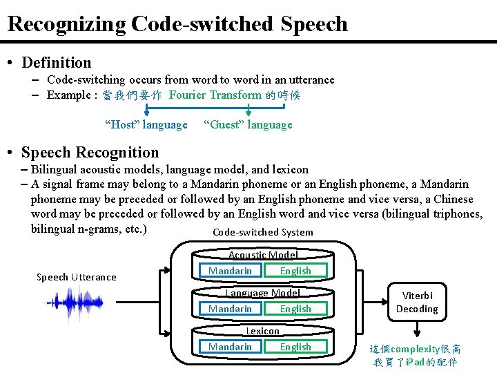
Recognizing Code-switched Speech • Definition – Code-switching occurs from word to word in an utterance – Example : 當我們要作 Fourier Transform 的時候 “Host” language “Guest” language • Speech Recognition – Bilingual acoustic models, language model, and lexicon – A signal frame may belong to a Mandarin phoneme or an English phoneme, a Mandarin phoneme may be preceded or followed by an English phoneme and vice versa, a Chinese word may be preceded or followed by an English word and vice versa (bilingual triphones, bilingual n-grams, etc. ) Code-switched System Speech Utterance Acoustic Model Mandarin English Language Model Mandarin English Lexicon Mandarin English Viterbi Decoding 這個complexity很高 我買了i. Pad的配件

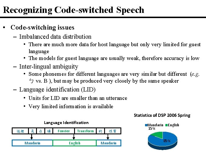
Recognizing Code-switched Speech • Code-switching issues – Imbalanced data distribution • There are much more data for host language but only very limited for guest language • The models for guest language are usually weak, therefore accuracy is low – Inter-lingual ambiguity • Some phonemes for different languages are very similar but different (e. g. ㄅ vs. B ), but may be produced very closely by the same speaker – Language identification (LID) • Units for LID are smaller than an utterance • Very limited information is available Statistics of DSP 2006 Spring Language Identification 這裡 是 在 Mandarin 講 Fourier Transform English 的 性質 Mandarin 15% English 85%

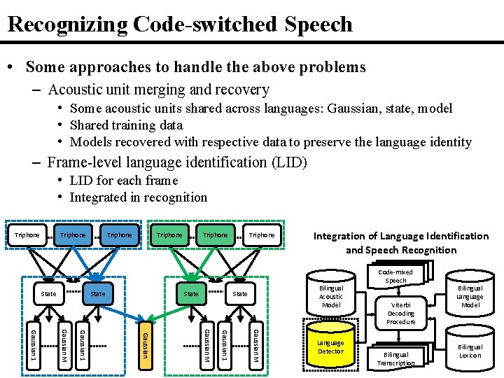
Recognizing Code-switched Speech • Some approaches to handle the above problems – Acoustic unit merging and recovery • Some acoustic units shared across languages: Gaussian, state, model • Shared training data • Models recovered with respective data to preserve the language identity – Frame-level language identification (LID) • LID for each frame • Integrated in recognition Triphone State Triphone Integration of Language Identification and Speech Recognition Bilingual Acoustic Model State Gaussian M Gaussian 1 Language Detector Code-mixed Speech Viterbi Decoding Procedure Bilingual Transcription Bilingual Language Model Bilingual Lexicon

References for Recognizing Code-switched Speech 1. “An Improved Framework for Recognizing Highly Imbalanced Bilingual Code-Switched Lectures with Cross-Language Acoustic Modeling and Frame-Level Language Identification”, IEEE/ACM Transactions on Audio, Speech and Language Processing, Vol. 23, No. 7, 2015. 2. “Recognition Of Highly Imbalanced Code-mixed Bilin-gual Speech With Frame-level Language Detection Based On Blurred Posteriorgram, ” ICASSP, 2012. 3. “Language Independent And Language Adaptive Acoustic Modeling For Speech Recognition, ” Tanja Schultz and Alex Waibel, Speech Communication, 2001. 4. “Learning Methods In Multilingual Speech Recognition, ” Hui Lin, Li Deng, Jasha Droppo, Dong Yu, and Alex Acero, NIPS, 2008.

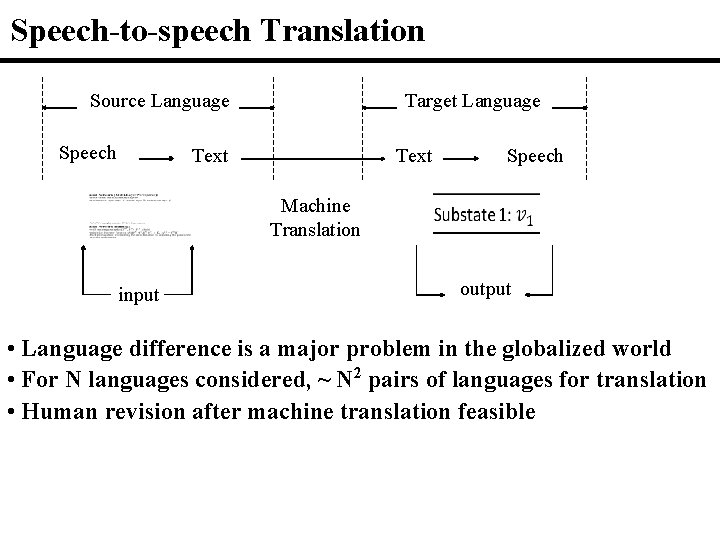
Speech-to-speech Translation Source Language Speech Target Language Text Speech Machine Translation input output • Language difference is a major problem in the globalized world • For N languages considered, ~ N 2 pairs of languages for translation • Human revision after machine translation feasible

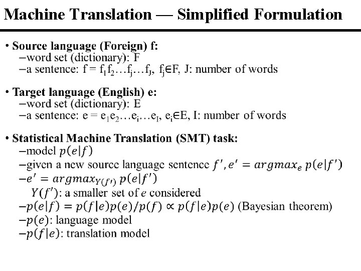
Machine Translation — Simplified Formulation •

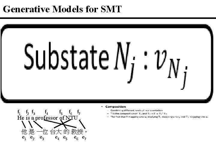
Generative Models for SMT • f 1 f 2 f 3 f 4 f 5 f 6 f 7 He is a professor of NTU. 他 是 一位 台大 的 教授。 e 1 e 2 e 3 e 4 e 5 e 6 e 7

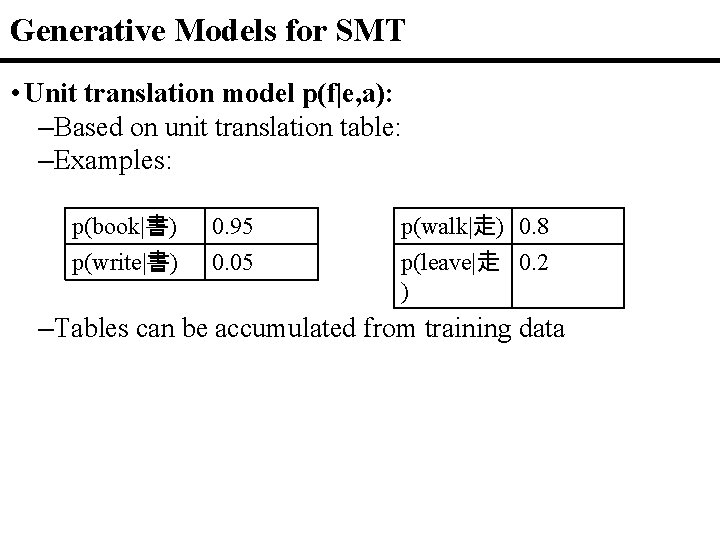
Generative Models for SMT • Unit translation model p(f|e, a): –Based on unit translation table: –Examples: p(book|書) p(write|書) 0. 95 0. 05 p(walk|走) 0. 8 p(leave|走 0. 2 ) –Tables can be accumulated from training data

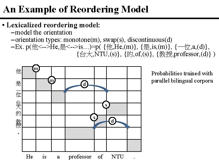
An Example of Reordering Model • Lexicalized reordering model: – model the orientation – orientation types: monotone(m), swap(s), discontinuous(d) – Ex. p(他<-->He, 是<-->is…)=p( {他, He, (m)}, {是, is, (m)}, {一位, a, (d)}, {台大, NTU, (s)}, {的, of, (s)}, {教授, professor, (d)} ) 他 是 一 位 台 大 的 教 授 。 m m Probabilities trained with parallel bilingual corpora d s s d He is a professor of NTU .

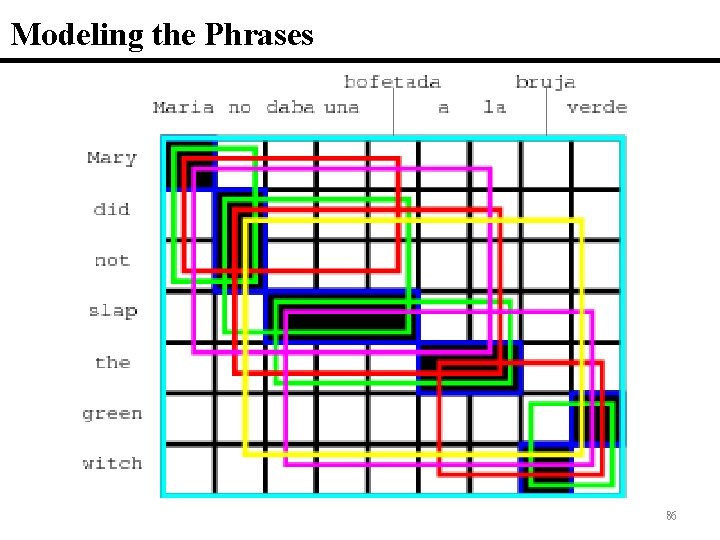
Modeling the Phrases 86

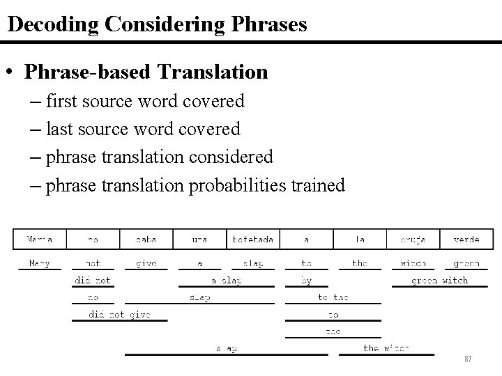
Decoding Considering Phrases • Phrase-based Translation – first source word covered – last source word covered – phrase translation considered – phrase translation probabilities trained 87

References for Translation • A Survey of Statistical Machine Translation – Adam Lopez – Tech. report of Univ. of Maryland • Statistical Machine Translation – Philipp Koehn – Cambridge University Press • Building a Phrase-based Machine Translation System – Kevin Duh and Graham Neubig – Lecture note of “Statistical Machine Translation, ” NAIST, 2012 spring • Speech Recognition, Machine Translation, and Speech Translation ‒ A Unified Discriminative Learning Paradigm – IEEE Signal Processing Magazine, Sept 2011 • Moses: Open Source Toolkit for Statistical Machine Translation – Annual Meeting of the Association for Computational Linguistics (ACL) demonstration session, Prague, Czech Republic, June 2007

References for Speech Recognition Updates • “Structured Discriminative Models for Speech Recognition”, IEEE Signal Processing Magazine, Nov 2012 • “Subword Modeling for Automatic Speech Recognition”, IEEE Signal Processing Magazine, Nov 2012 • “Machine Learning Paradigms for Speech Recognition ‒ An Overview”, IEEE Transactions on Audio, Speech and Language Processing, May 2013