9 0 Laplace Transform 9 1 General Principles


 jω Fourier transform")

 may not be well")


 l Property 1 : ROC of X(s) consists of strips")

 l Property 3 : If x(t) is of finite duration")
 l Property 4 : If x(t) is right-sided (x(t)=0, t")

 l Property 5 : If x(t) is left-sided (x(t)=0, t")

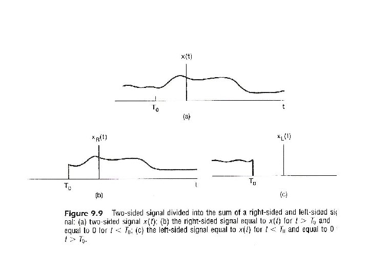
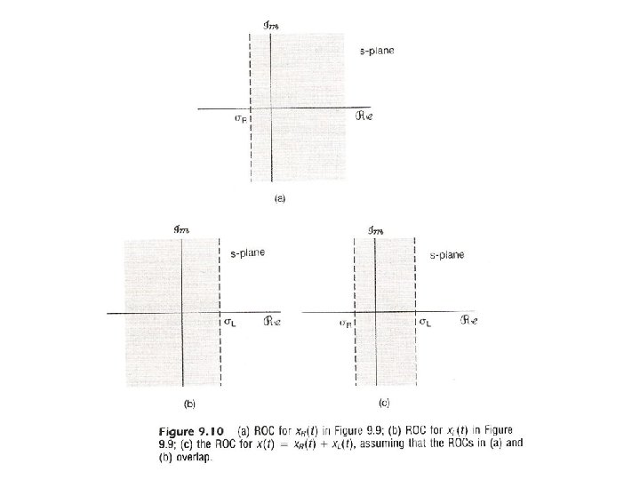
 l Property 6 : If x(t) is two-sided, and {s")
 l A signal or an impulse response either doesn’t have")
 l Property 7 : If X(s) is rational, then its")
 l Property 8 : If x(s) is rational, then if")

 l An expression of X(s) may corresponds to different signals")

![Inverse Laplace Transform – integration along a line {s | Re[s]=σ1} ROC for a](https://slidetodoc.com/presentation_image/4810a2ca08db755e23e3e8eb555edc7e/image-28.jpg "Inverse Laplace Transform – integration along a line {s | Re[s]=σ1} ROC for a")
 X (合成 ? ) X (分析 ? ) X (分析)")


 – Expansion (? ) of")
 is real, and X(s) has a pole/zero at then")


 = 0, t < 0 x(t) has no")
=x(t)*h(t) x(t) h(t) X(s) H(s) system function")
 whose ROC is a righthalf")

")


 = h 1(t) + h 2(t) H(s)")
 + - + e(t) h 1(t) H")

u is always a right-half plane – a causal h(t) has")


- Slides: 63
9. 0 Laplace Transform 9. 1 General Principles of Laplace Transform l Eigenfunction Property x(t) = est h(t) linear time-invariant y(t) = H(s)est
Chapters 3, 4, 5, 9, 10 Chap 3 Chap 4 Chap 5 Chap 9 jω Chap 10
Laplace Transform l Eigenfunction Property eigenfunction of all linear time-invariant systems with unit impulse response h(t) – applies for all complex variables s Fourier Transform Laplace Transform
Laplace Transform l A Generalization of Fourier Transform X( + jω) jω Fourier transform of
Laplace Transform
Laplace Transform l A Generalization of Fourier Transform – X(s) may not be well defined (or converged) for all s – X(s) may converge at some region of s-plane, while x(t) doesn’t have Fourier Transform – covering broader class of signals, performing more analysis for signals/systems
Laplace Transform l Rational Expressions and Poles/Zeros roots zeros roots poles – Pole-Zero Plots – specifying X(s) except for a scale factor
Laplace Transform l Rational Expressions and Poles/Zeros – Geometric evaluation of Fourier/Laplace transform from pole-zero plots each term (s-βi) or (s-αj) represented by a vector with magnitude/phase
Poles & Zeros x x
Region of Convergence (ROC) l Property 1 : ROC of X(s) consists of strips parallel to the jω -axis in the s-plane – For the Fourier Transform of x(t)e-σt to converge depending on σ only l Property 2 : ROC of X(s) doesn’t include any poles
Property 1, 3
Region of Convergence (ROC) l Property 3 : If x(t) is of finite duration and absolutely integrable, the ROC is the entire s-plane
Region of Convergence (ROC) l Property 4 : If x(t) is right-sided (x(t)=0, t < T 1), and {s | Re[s] = σ0} ROC, then {s | Re[s] > σ0} ROC, i. e. , ROC includes a right-half plane
Property 4
Region of Convergence (ROC) l Property 5 : If x(t) is left-sided (x(t)=0, t > T 2), and {s | Re[s] = σ0} ROC, then {s | Re[s] < σ0} ROC, i. e. , ROC includes a left-half plane
Property 5
Region of Convergence (ROC) l Property 6 : If x(t) is two-sided, and {s | Re[s] = σ0} ROC, then ROC consists of a strip in s-plane including {s | Re[s] = σ0} See Fig. 9. 9, 9. 10, p. 667 of text *note: ROC[x(t)] may not exist
Region of Convergence (ROC) l A signal or an impulse response either doesn’t have a Laplace Transform, or falls into the 4 categories of Properties 3 -6. Thus the ROC can be , s-plane, lefthalf plane, right-half plane, or a single strip
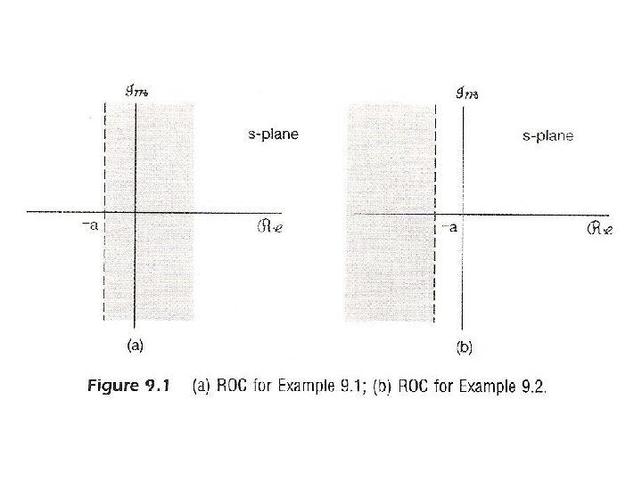
Region of Convergence (ROC) l Property 7 : If X(s) is rational, then its ROC is bounded by poles or extends to infinity – examples: See Fig. 9. 1, p. 658 of text – partial-fraction expansion
Region of Convergence (ROC) l Property 8 : If x(s) is rational, then if x(t) is rightsided, its ROC is the right-half plane to the right of the rightmost pole. If x(t) is left-sided, its ROC is the left-half plane to the left of the leftmost pole.
Property 8 ROC
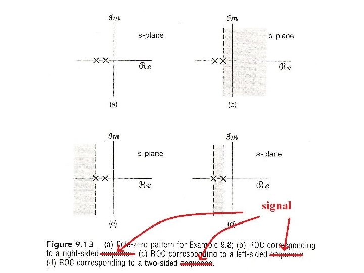
Region of Convergence (ROC) l An expression of X(s) may corresponds to different signals with different ROC’s. – an example: See Fig. 9. 13, p. 670 of text – ROC is a part of the specification of X(s) l The ROC of X(s) can be constructed using these properties
ROC and Poles/Zeros
Inverse Laplace Transform – integration along a line {s | Re[s]=σ1} ROC for a fixed σ1
Laplace Transform (basis? ) X (合成 ? ) X (分析 ? ) X (分析) basis (合成) (分析)
Inverse Laplace Transform l Practically in many cases : partial-fraction expansion works , ROC – ROC to the right of the pole at s = -ai – ROC to the left of the pole at s = -ai l Known pairs/properties practically helpful
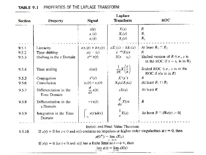
9. 2 Properties of Laplace Transform l Linearity l Time Shift
Time Shift
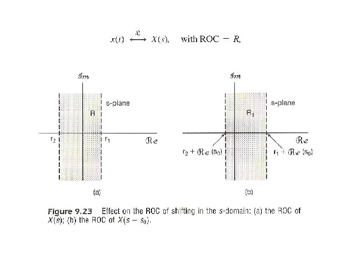
l Shift in s-plane See Fig. 9. 23, p. 685 of text – for s 0 = jω0 shift along the jω axis
Shift in s-plane
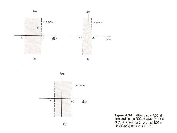
l Time Scaling (error on text corrected in class) – Expansion (? ) of ROC if a > 1 Compression (? ) of ROC if 1 > a > 0 reversal of ROC about jw-axis if a < 0 (right-sided left-sided, etc. ) See Fig. 9. 24, p. 686 of text
l Conjugation – if x(t) is real, and X(s) has a pole/zero at then X(s) has a pole/zero at l Convolution – ROC may become larger if pole-zero cancellation occurs
l Differentiation ROC may become larger if a pole at s = 0 cancelled
l Integration in time Domain
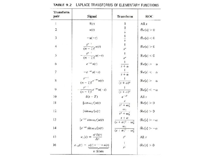
l Initial/Final – Value Theorems x(t) = 0, t < 0 x(t) has no impulses or higher order singularities at t = 0 l Tables of Properties/Pairs See Tables 9. 1, 9. 2, p. 691, 692 of text
9. 3 System Characterization with Laplace Transform y(t)=x(t)*h(t) x(t) h(t) X(s) H(s) system function transfer function Y(s)=X(s)H(s)
l Causality – A causal system has an H(s) whose ROC is a righthalf plane h(t) is right-sided – For a system with a rational H(s), causality is equivalent to its ROC being the right-half plane to the right of the rightmost pole – Anticausality a system is anticausal if h(t) = 0, t > 0 an anticausal system has an H(s) whose ROC is a left -half plane, etc.
Causality right-sided X ROC is right half Plane Causal
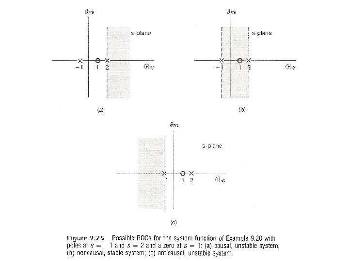
l Stability – A system is stable if and only if ROC of H(s) includes the jω -axis h(t) absolutely integrable, or Fourier transform converges See Fig. 9. 25, p. 696 of text – A causal system with a rational H(s) is stable if and only if all poles of H(s) lie in the left-half of s-plane ROC is to the right of the rightmost pole
Stability
l Systems Characterized by Differential Equations zeros poles
l System Function Algebra – Parallel h(t) = h 1(t) + h 2(t) H(s) = H 1(s) + H 2(s) – Cascade h(t) = h 1(t) * h 2(t) H(s) = H 1(s)‧ H 2(s)
l System Function Algebra – Feedback x(t) + - + e(t) h 1(t) H 1(s) z(t) h 2(t) H 2(s) y(t)
9. 4 Unilateral Laplace Transform impulses or higher order singularities at t = 0 included in the integration
– ROC for X(s)u is always a right-half plane – a causal h(t) has H(s) = H(s) – two signals differing for t < 0 but identical for t ≥ 0 have identical unilateral Laplace transforms – similar properties and applications
Examples • Example 9. 7, p. 668 of text
Examples • Example 9. 7, p. 668 of text b>0
Examples • Example 9. 9/9. 10/9. 11, p. 671 -673 of text
Examples • Example 9. 9/9. 10/9. 11, p. 671 -673 of text
Examples • Example 9. 25, p. 701 of text left-half plane
Problem 9. 60, p. 737 of text Echo in telephone communication
Problem 9. 60, p. 737 of text zeros
Problem 9. 60, p. 737 of text
Problem 9. 44, p. 733 of text