8 Speech Recognition Speech Recognition Concepts Speech Recognition

8 -Speech Recognition � Speech Recognition Concepts � Speech Recognition Approaches � Recognition Theories � Bayse Rule � Simple Language Model � P(A|W) Network Types 1

7 -Speech Recognition (Cont’d) � HMM Calculating Approaches � Neural Components � Three Basic HMM Problems � Viterbi Algorithm � State Duration Modeling � Training In HMM 2

Recognition Tasks Isolated Word Recognition (IWR) Connected Word (CW) , And Continuous Speech Recognition (CSR) � Speaker Dependent, Multiple Speaker, And Speaker Independent � Vocabulary Size � �Small <20 �Medium >100 , <1000 �Large >1000, <10000 �Very Large >10000 3

Speech Recognition Concepts Speech recognition is inverse of Speech Synthesis Text Speech Phone Processing Sequence NLP Speech Processing Text Speech Understanding Speech Recognition 4

Speech Recognition Approaches � Bottom-Up Approach � Top-Down Approach � Blackboard Approach 5

Bottom-Up Approach Signal Processing Knowledge Sources Feature Extraction Voiced/Unvoiced/Silence Segmentation Signal Processing Sound Classification Rules Feature Extraction Phonotactic Rules Segmentation Lexical Access Language Model Segmentation Recognized Utterance 6

Top-Down Approach Inventory Word of speech Dictionary Grammar recognition units Feature Analysis Syntactic Hypo thesis Unit Matching System Lexical Hypo thesis Utterance Verifier/ Matcher Recognized Utterance Task Model Semantic Hypo thesis 7

Blackboard Approach Acoustic Processes Environmental Processes Lexical Processes Black board Semantic Processes Syntactic Processes 8

Recognition Theories Articulatory Based Recognition �Use Articulatory system modeling for recognition �This theory is the most successful so far � Auditory Based Recognition �Use Auditory system for recognition � Hybrid Based Recognition �Is a combination of the above theories � Motor Theory �Model the intended gesture of speaker � 9

Recognition Problem � We have the sequence of acoustic symbols and we want to find the words uttered by speaker � Solution : Find the most probable word sequence given Acoustic symbols 10

Recognition Problem �A : Acoustic Symbols � W : Word Sequence � we should find so that 11

Bayse Rule 12

Bayse Rule (Cont’d) 13

Simple Language Model Computing this probability is very difficult and we need a very big database. So we use Trigram and Bigram models. 14

Simple Language Model (Cont’d) Trigram : Bigram : Monogram : 15

Simple Language Model (Cont’d) Computing Method : Number of happening W 3 after W 1 W 2 Total number of happening W 1 W 2 Ad hoc Method : 16

Error Production Factor � Prosody (Recognition should be Prosody Independent) � Noise (Noise should be prevented) � Spontaneous Speech 17

P(A|W) Computing Approaches � Dynamic � Hidden Markov Model (HMM) � Artificial � Hybrid Time Warping (DTW) Neural Network (ANN) Systems 18

Dynamic Time Warping 19

Dynamic Time Warping 20

Dynamic Time Warping 21

Dynamic Time Warping 22

Dynamic Time Warping Search Limitation : - First & End Interval - Global Limitation - Local Limitation 23

Dynamic Time Warping Global Limitation : 24

Dynamic Time Warping Local Limitation : 25

Artificial Neural Network . . . Simple Computation Element of a Neural Network 26

Artificial Neural Network (Cont’d) � Neural Network Types �Perceptron �Time Delay Neural Network Computational Element (TDNN) 27

Artificial Neural Network (Cont’d) Single Layer Perceptron. . . 28

Artificial Neural Network (Cont’d) Three Layer Perceptron. . . 29

2. 5. 4. 2 Neural Network Topologies 30

TDNN 31

2. 5. 4. 6 Neural Network Structures for Speech Recognition 32

es for Speech Recognition 33

Hybrid Methods Hybrid Neural Network and Matched Filter For Recognition Acoustic Output Units Speech Features Delays � PATTERN CLASSIFIER 34

Neural Network Properties � The system is simple, But too much iteration is needed for training � Doesn’t determine a specific structure � Regardless of simplicity, the results are good � Training size is large, so training should be offline 35

Pre-processing � Different preprocessing techniques are employed as the front end for speech recognition systems � The choice of preprocessing method is based on the task, the noise level, the modeling tool, etc. 36

37

38

39

40

41

42

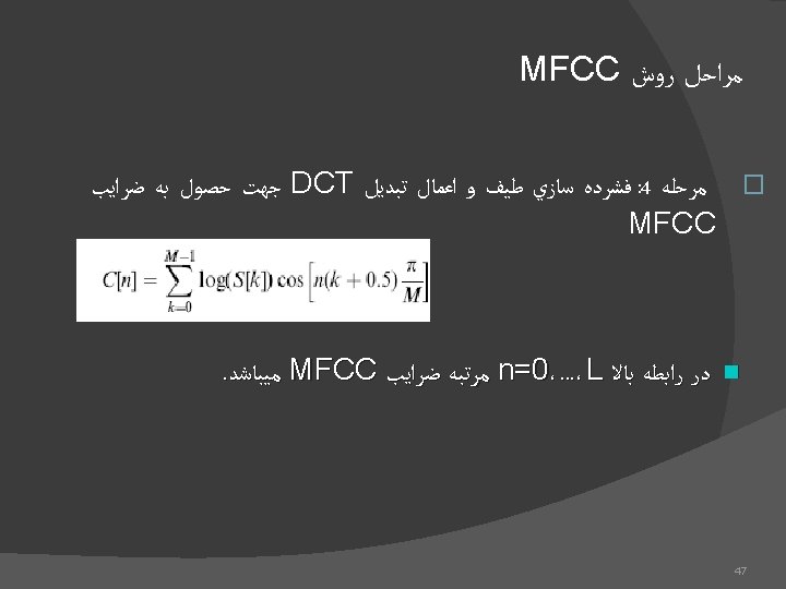
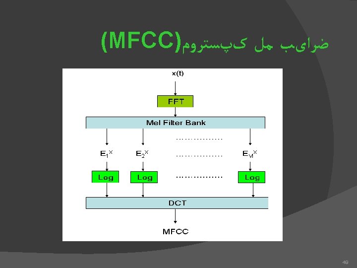
کپﺴﺘﺮﻭﻡ - ﺭﻭﺵ ﻣﻞ ﺳﻴگﻨﺎﻝ ﺯﻣﺎﻧی ﻓﺮیﻢ ﺑﻨﺪی |FFT|2 Mel-scaling Logarithm IDCT Cepstra Delta & Delta Cepstra Differentiator 48 Low-order coefficients

Time-Frequency analysis � Short-term Fourier Transform � Standard way of frequency analysis: decompose the incoming signal into the constituent frequency components. � W(n): windowing function � N: frame length � p: step size 51

Critical band integration � Related to masking phenomenon: the threshold of a sinusoid is elevated when its frequency is close to the center frequency of a narrow-band noise � Frequency components within a critical band are not resolved. Auditory system interprets the signals within a critical band as a whole 52

Bark scale 53

Feature orthogonalization � Spectral values in adjacent frequency channels are highly correlated � The correlation results in a Gaussian model with lots of parameters: have to estimate all the elements of the covariance matrix � Decorrelation is useful to improve the parameter estimation. 54

Cepstrum � Computed as the inverse Fourier transform of the log magnitude of the Fourier transform of the signal The log magnitude is real and symmetric -> the transform is equivalent to the Discrete Cosine Transform. � Approximately decorrelated � 55

Principal Component Analysis Find an orthogonal basis such that the reconstruction error over the training set is minimized � This turns out to be equivalent to diagonalize the sample autocovariance matrix � Complete decorrelation � Computes the principal dimensions of variability, but not necessarily provide the optimal discrimination among classes � 56

Principal Component Analysis (PCA) � Mathematical procedure that transforms a number of (possibly) correlated variables into a (smaller) number of uncorrelated variables called principal components (PC) � Find an orthogonal basis such that the reconstruction error over the training set is minimized � This turns out to be equivalent to diagonalize the sample autocovariance matrix � Complete decorrelation � Computes the principal dimensions of variability, but not necessarily provide the optimal discrimination among classes 57

PCA (Cont. ) � Algorithm Input= Covariance matrix (N-dim vectors) Output = (R- dim vectors) Eigen values Eigen vectors Transform matrix Apply Transform 58

PCA (Cont. ) � PCA in speech recognition systems 59

Linear discriminant Analysis � Find an orthogonal basis such that the ratio of the between-class variance and within-class variance is maximized � This also turns to be a general eigenvalueeigenvector problem � Complete decorrelation � Provide the optimal linear separability under quite restrict assumption 60

PCA vs. LDA 61

Spectral smoothing � Formant information is crucial for recognition � Enhance and preserve the formant information: �Truncating the number of cepstral coefficients �Linear prediction: peak-hugging property 62

Temporal processing � To capture the temporal features of the spectral envelop; to provide the robustness: �Delta Feature: first and second order differences; regression �Cepstral Mean Subtraction: ○ For normalizing for channel effects and adjusting for spectral slope 63

RASTA (Rel. Ative Spec. Tral Analysis) �Filtering of the temporal trajectories of some function of each of the spectral values; to provide more reliable spectral features �This is usually a bandpass filter, maintaining the linguistically important spectral envelop modulation (1 -16 Hz) 64

65

RASTA-PLP 66

67

68

Language Models for LVCSR Word Pair Model: Specify which word pairs are valid 69

Statistical Language Modeling 70

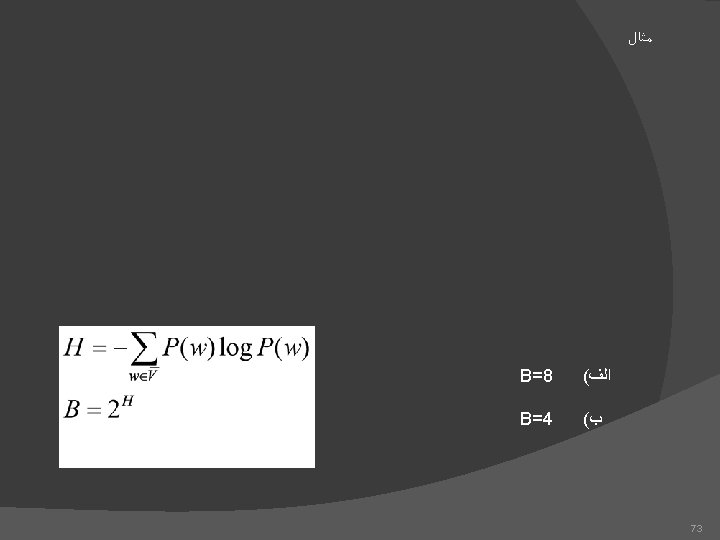
Perplexity of the Language Model Entropy of the Source: Assuming independence: First order entropy of the source: If the source is ergodic, meaning its statistical properties can be completely characterized in a sufficiently long sequence that the source puts out, 71

We often compute H based on a finite but sufficiently large Q: H is the degree of difficulty that the recognizer encounters, on average, When it is to determine a word from the same source. Using language model, if the N-gram language model PN(W) is used, An estimate of H is: In general: Perplexity is defined as: 72

Overall recognition system based on subword units 74