8 Solution of Linear Differential Equations Example 8

8. Solution of Linear Differential Equations: Example 8. 1 Transfer Function: f(t): Input, u(t): Output If f(t)=est then u(t)= H(s)est where H(s) is the transfer function which transforms the input to the output s 3 H(s)est+4 s 2 H(s)est+14 s. H(s)est+20 H(s)est=3 est+sest (s 3+4 s 2+14 s+20)H(s)=3+s a=[1, 4, 14, 20]; roots(a) Eigenvalues: -1± 3 i, -2 Exponential/Harmonic Input: s=-0. 2+2. 7 i; hs=(s+3)/(s^3+4*s^2+14*s+20); abs(hs), angle(hs) RESONANCE

Laplace Transform: x(t) H(s) y(t) Y(s)=X(s) H(s)

1 0 Δ(s)=1 u(t): Unit step function Impulse function Magnitude of the step input Final value theorem:

Impulse Response: Inverse Laplace transform of H(s) a=[1, 4, 14, 20]; roots(a) Eigenvalues: -1± 3 i, -2 (Partial fraction expansion): p 1=[1, 3]; p 2=[1, 4, 14, 20]; [r, p, k]=residue(p 1, p 2) r(1)=-0. 05 -0. 1833 i, r(2)=-0. 05+0. 1833 i, r(3)=0. 1 z=-0. 05+0. 1833 i 2*abs(z) phase(z) ξ=0. 3162 (s=-1± 3 i), suitable values of Δt=0. 099 and t∞=6. 283

ξ=0. 3162 (s=-1± 3 i), use Δt=0. 099 and t∞=6. 283 to plot the response h(t) clc; clear; t=0: 0. 099: 6. 283; yt=0. 3801*exp(-t). *cos(3*t-1. 837)+0. 1*exp(-2*t) plot(t, yt)

Step Input Response: y(t) Inverse Laplace Transform of Y(s) Singular Points (Eigenvalues) are -1± 3 i , -2 and s=0 Partial fraction expansion: p 1=[1, 3]; p 2=[1, 4, 14, 20, 0]; [r, p, k]=residue(p 1, p 2) r(1)=-0. 05+0. 0333 i, r(2)=-0. 05 -. 0033 i, r(3)=-0. 05, r(4)=0. 15 Final value theorem: yss=0. 15

clc; clear; t=0: 0. 099: 6. 283; yt=0. 1202*exp(-t). *cos(3*t+2. 5536)-0. 05*exp(-2*t)+0. 15; plot(t, yt)

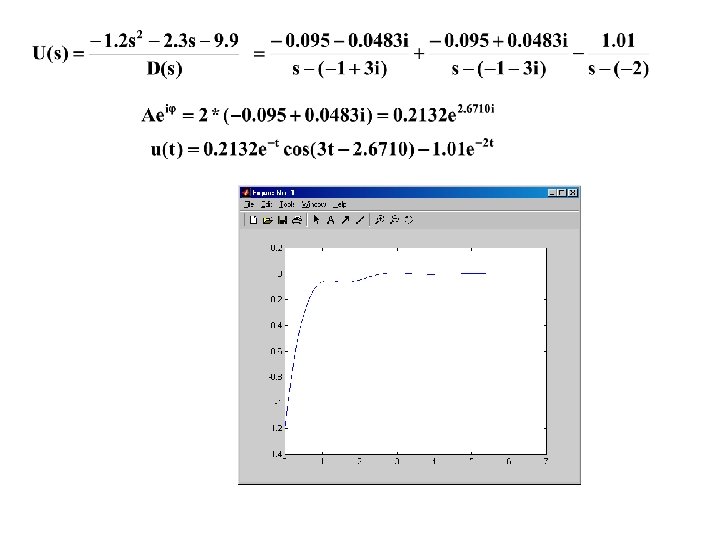
Solution due to the Initial Conditions (Homogeneous Solution): f=0 t=0 da p 1=[-1. 2, -2. 3, -9. 9]; p 2=[1, 4, 14, 20]; [r, p, k]=residue(p 1, p 2) r(1)=-0. 095 -0. 0483 i, r(2)=-0. 095+0. 0483 i, r(3)=-1. 01

Problem: m 1 , L 1 m 2 k c θ y. A For the mechanical sysem given in the figure, y. A is input and θ is output. Take m 1=250 kg, m 2=350 kg, k=37000 N/m, c=1500 Ns/m and L 1=1. 2 m. The governing differential equation of the system is given as a) Find the output θ(t) for y. A(t)=0. 2 e-3 tcos(17 t-1. 8) Solution: y. A(t)=est and θ(t)= H(s)est s=-3+17 i ; h=(1800*s+44400)/(624*s^2+2160*s+53280) abs(h) angle(h)